
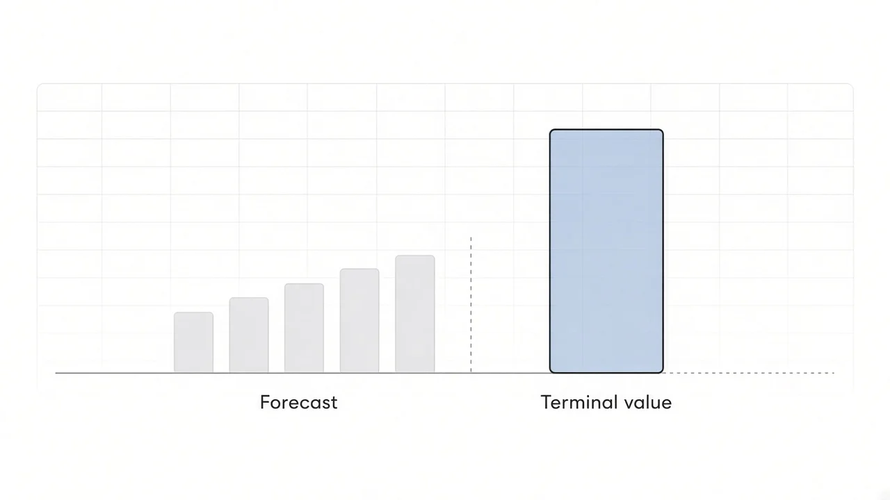
Terminal value is the value of a business's cash flows beyond the last year an analyst forecasts in detail, expressed as a single amount at the end of that forecast. In a discounted cash flow (DCF) valuation it is calculated one of two ways, either by growing the final year's free cash flow at a constant rate forever, the perpetuity growth method, or by applying a valuation multiple such as enterprise value to earnings before interest, taxes, depreciation and amortization (EBITDA) to the final year's earnings, the exit multiple method. Because it stands in for every year after the forecast, terminal value usually accounts for most of a DCF's result, and sometimes all of it. When the special committee of WideOpenWest, a US broadband provider, weighed a 2025 take-private by DigitalBridge and Crestview Partners, its adviser Centerview Partners valued the same management plan both ways. In February 2025 it used perpetuity growth of 2.5% to 3.0%, which implied exit multiples of 5.2 to 7.0 times terminal-year EBITDA. In August it used exit multiples of 5.0 to 6.0 times, which implied growth of 0.8% to 2.9%. In both analyses the discounted terminal value was slightly more than the company's entire enterprise value.
What terminal value is
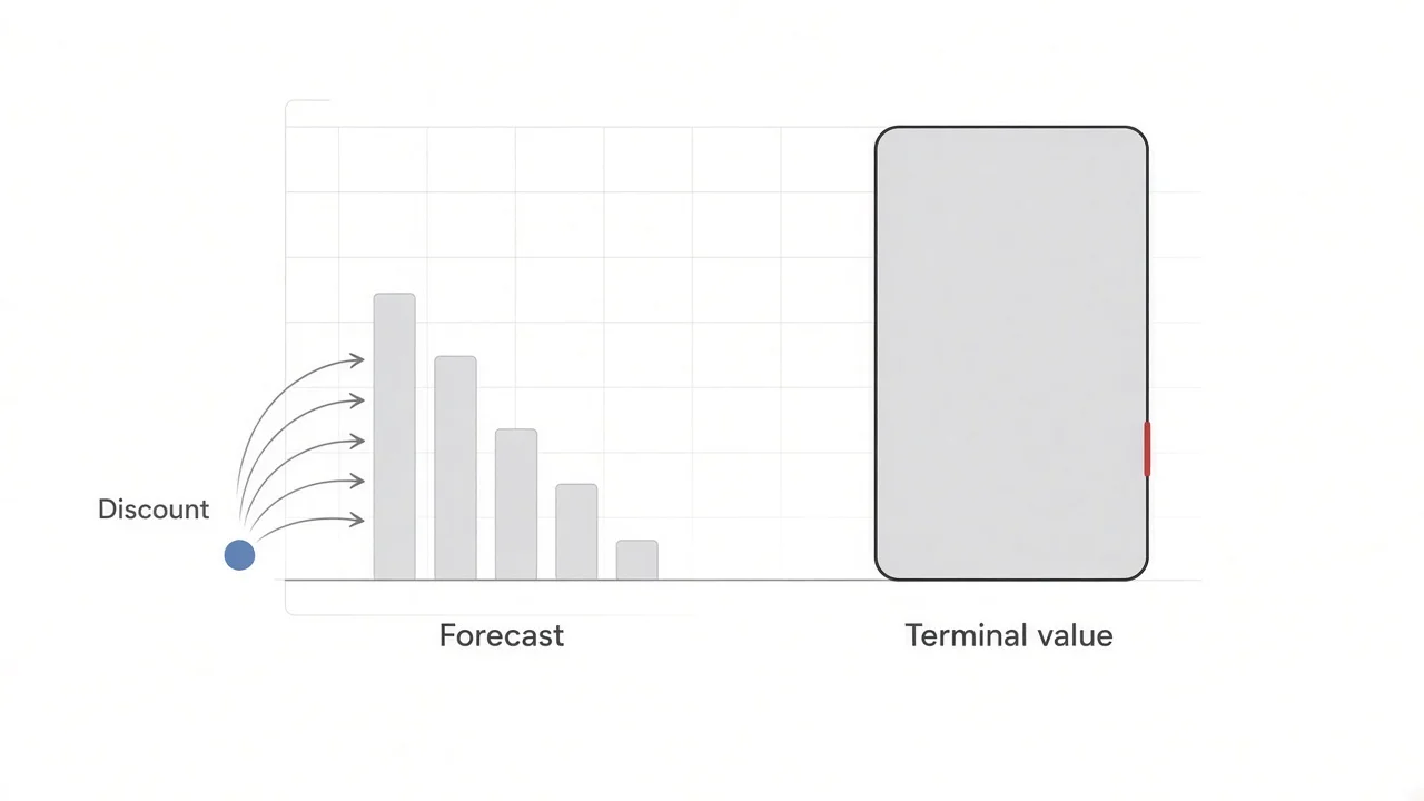
A DCF values a company at the present value of all the cash it will generate. No one can forecast a company year by year forever, so the analysis has two stages. The first is an explicit forecast, usually five to ten years, in which revenue, margins, capital spending and working capital are modeled line by line. The second is the terminal value, which captures everything after that in one figure. Terminal value is also called continuing value or horizon value. It is calculated as of the end of the forecast, so a five-year model produces a terminal value at the end of year five, which is then discounted to today along with the forecast cash flows.
The terminal value assumes the business keeps operating as a going concern. If it will not, because a mine runs out, a license expires or a fund winds down, the right closing figure is a liquidation or salvage value instead, the cash the assets would bring in a sale. Aswath Damodaran of NYU Stern lists liquidation value as the third way to close a valuation, alongside the perpetuity growth and multiple methods, in his paper "Closure in Valuation: Estimating Terminal Value". He estimates liquidation value in one of two ways: from the book value of the assets in the terminal year, adjusted for inflation over their average age, or from the present value of the cash the assets will still produce over their remaining life. In an equity valuation, the debt outstanding in the terminal year is then subtracted.
What the terminal value represents depends on the cash flow being valued:
- Unlevered free cash flow (cash available to both lenders and shareholders), discounted at the weighted average cost of capital (WACC), gives a terminal value of the whole enterprise. This is the standard build in banking and private equity.
- Levered free cash flow (cash left for shareholders after interest and debt repayment), discounted at the cost of equity, gives a terminal value of equity only.
Mixing the two, for example discounting unlevered cash flow at the cost of equity, produces a number that is neither.
Terminal value is large because it covers far more years than the forecast does. For a company whose free cash flow grows 3% a year forever, discounted at 9%, a dollar received in year 30 is worth about 8 cents today (1 / 1.09^30 = 0.075), yet the years after year five still account for 75% of the company's value, and the years after year ten for 57%. For a company that is still investing heavily, the share can exceed 100%, because the forecast years together are worth little or less than nothing. WideOpenWest, which planned to spend most of its EBITDA on capital projects through 2027, including new fiber markets, is an example.
Terminal value formulas
Perpetuity growth method
Terminal value = FCF(n) × (1 + g) / (WACC − g)
- FCF(n) is unlevered free cash flow in the final forecast year. Multiplying by (1 + g) gives the first year after the forecast, which is the cash flow the formula needs.
- g is the constant rate at which free cash flow grows forever.
- WACC is the discount rate. It must be higher than g, or the formula produces a negative or infinite value.
The formula is the value of a growing perpetuity, and it is also called the Gordon growth model, after Myron Gordon, a University of Toronto economist who applied the same arithmetic to dividends in a 1959 paper. A company with final-year free cash flow of $100 million, 3% growth and a 9% WACC has a terminal value of $100 million × 1.03 / 0.06, or about $1,717 million. At 2% growth the figure is $1,457 million, and at 4% it is $2,080 million. The closer g gets to the discount rate, the faster the value rises.
Two variants appear in practice. Setting g to zero gives FCF(n) / WACC, a conservative closing value that analysts sometimes use when the growth rate is hard to estimate. A multi-stage version lets growth fade over a second forecast period, for example from 8% to 3% over five years, before the perpetuity begins, which suits companies that are still growing fast at the end of the explicit forecast.
Exit multiple method
Terminal value = final-year metric × exit multiple
The metric is usually EBITDA, and the multiple is an enterprise value multiple taken from comparable companies or precedent transactions. The same company, with final-year EBITDA of $200 million and an exit multiple of 8.0 times, has a terminal value of $1,600 million. Revenue, EBIT and, for banks and insurers, book value or earnings multiples are used where EBITDA does not describe the business.
Present value of terminal value
Present value of terminal value = terminal value / (1 + WACC)^n
Both methods give a value as of the end of year n, so it is discounted with the same factor as a cash flow received at that date. At 9% over five years the factor is 0.650, which turns $1,717 million into about $1,116 million and $1,600 million into about $1,040 million. Enterprise value is the sum of that figure and the present value of the forecast cash flows.
How to calculate terminal value, step by step
- Make the final forecast year a steady state. The terminal value repeats the last year forever, so that year has to look like the business in maturity. Revenue growth should be close to the terminal growth rate, margins should have stopped expanding, capital spending should cover maintenance plus the investment that growth requires, and working capital should be at a normal level. Taxes should be at the long-run rate. Tax losses that will run out are valued separately, as Centerview did for WideOpenWest's net operating losses. The year should not sit at a cyclical peak or trough, and the EBITDA an exit multiple is applied to should exclude one-time costs and, in a private company, owners' personal expenses. If the last year is not representative, add a normalized terminal year after it.
- Choose the method and its input. For perpetuity growth, pick a long-run nominal growth rate. For an exit multiple, pick a multiple from trading or deal data for mature companies like the one being valued, and make sure it is measured on the same metric, before or after stock-based compensation, that you apply it to.
- Calculate the terminal value with the formula for that method, using the full final year of cash flow or EBITDA. A common modeling error is to take only the last quarter or month.
- Discount it to the valuation date. With year-end discounting, divide by (1 + WACC)^n. With the mid-year convention, which assumes cash arrives evenly through each year, the forecast cash flows are discounted from mid-year. The terminal value then needs care. An exit multiple is a sale price at the end of year n and is still discounted over n years, while a perpetuity growth value is usually multiplied by (1 + WACC)^0.5 so that its cash flows are also treated as arriving mid-year. If the valuation date falls inside a year, the discount period is fractional. Centerview's August 2025 WideOpenWest analysis, with a valuation date of June 30, 2025, discounted a terminal value at the end of 2029 over 4.5 years.
- Cross-check it with the other method. Calculate the exit multiple implied by a perpetuity growth value, or the growth rate implied by an exit multiple, and ask whether the result is believable.
- Run a sensitivity table of value across discount rates and growth rates or multiples. Bankers present the result as a range.
- Add the present value of the forecast cash flows to get enterprise value, then subtract net debt and add any separately valued items, such as tax loss carryforwards, to reach equity value.
The mid-year adjustment in step 4 is easy to miss and changes the answer. In the February 2025 WideOpenWest analysis, the midpoint (8.88% WACC, 2.75% growth) produced $5.86 a share with the adjustment and $5.16 without it, 12% less. The adjustment also changes the cross-check. The implied exit multiple at the midpoint is 5.95 times with it and 5.71 times without it. Centerview's slide shows 6.0 times, which matches only the adjusted figure.
Perpetuity growth method: choosing the growth rate
The growth rate in the formula is nominal, so it includes inflation, and it has to be in the same currency and on the same basis as the cash flows and the WACC. Because it applies forever, it cannot exceed the long-run growth of the economy the company sells into. A company that grew faster than the economy forever would eventually become the economy.
Damodaran's working rule is stricter. The stable growth rate should not exceed the risk-free rate used in the valuation, because over the long run the nominal risk-free rate tends toward the nominal growth rate of the economy. In a US valuation that means the 10-year Treasury yield, which the Treasury's daily par yield curve put at 4.54% on February 11, 2025, 4.27% on August 8, 2025 and 5.04% on November 19, 2026. Mature US companies are usually given growth well below that cap, and Centerview's WideOpenWest analyses used 2.5% to 3.5% in August 2024 and 2.5% to 3.0% in February 2025. Risk should settle down too. A company in stable growth should have close to average market risk, and Damodaran suggests that betas in the terminal period should not exceed about 1.2, so a fast-growing company's terminal WACC can be lower than its forecast-period WACC. Mature companies can also carry more debt, which lowers the WACC further, and Damodaran moves the debt ratio toward a sustainable level only if managers are likely to change it. A declining business can be given negative growth. In Damodaran's example, $100 million of after-tax cash flow shrinking 5% a year at a 10% cost of capital is worth $633 million, a business that liquidates itself a little each year.
Growth has to be paid for
The perpetuity formula takes free cash flow as given, but free cash flow and growth are linked. A company grows by reinvesting part of its after-tax operating profit (NOPAT), and the growth it gets depends on the return it earns on that reinvestment. The value-driver form of the formula, which Damodaran's paper builds on, makes the link explicit:
Terminal value = NOPAT(n+1) × (1 − g / RONIC) / (WACC − g)
RONIC is the return on new invested capital, and g / RONIC is the share of NOPAT that must be reinvested to grow at g. If new capital earns exactly the WACC, the growth adds no value and the terminal value collapses to NOPAT(n+1) / WACC, whatever g is. If RONIC is above the WACC, growth adds value; if it is below, growth destroys it. In his recorded lecture on terminal value, Damodaran says that for about 80% of companies he sets the return on capital in stable growth equal to the cost of capital, and for the one in five with large, durable competitive advantages he leaves it 2 or 3 points above.
WideOpenWest's terminal year shows why this matters. Centerview's normalized terminal year has capital spending equal to depreciation ($200 million each), no change in working capital, and free cash flow of $128 million against NOPAT of $132 million. Net reinvestment is zero, so the 2.75% midpoint growth comes free. Recomputing the February midpoint with the value-driver formula:
| Return on new capital | Share of NOPAT reinvested | Free cash flow, first year after the forecast | Change in terminal value | Value per share |
|---|---|---|---|---|
| Filed terminal year (capital spending equals depreciation) | 0% (other items take 3%) | $132m | none | $5.86 |
| 30% | 9% | $123m | −6% | $4.80 |
| 15% | 18% | $111m | −16% | $3.22 |
| 8.88% (equal to WACC) | 31% | $94m | −29% | $1.04 |
The filed assumption can be defended if the growth comes from price increases on a network that is already built, since raising prices takes little new capital. It is harder to defend if the growth requires extending the network to new homes, which takes new plant. The point applies to any terminal year in which capital spending equals depreciation, because such a model assumes that growth costs nothing.
For companies whose main investment is expensed, such as software, research or brands, reported returns on capital look high, because the intangible assets that produce the profit are not on the balance sheet. The return and the reinvestment in the formula have to be measured on the same basis. If the spending on intangibles stays in operating costs, the reinvestment in the model excludes it and the higher reported return is the consistent input. If the spending is capitalized, reinvestment rises and the return falls toward the cost of capital, a point The Footnotes Analyst works through in "DCF terminal values: Returns, growth and intangibles" (October 2021).
Exit multiple method: choosing the multiple
The exit multiple is the multiple a buyer or the market would pay for the business at the end of the forecast. Four choices decide it.
Trading or deal multiples. Multiples of public comparable companies reflect minority stakes traded on an exchange. Multiples from precedent transactions reflect purchases of whole companies and include a control premium, so they run higher. A DCF meant to show the company's standalone value normally uses trading multiples. A model that assumes the business is sold at the end of the forecast, as a buyout model does, can justify deal multiples, but the difference should be a decision rather than an accident. For private companies, appraisers often take deal multiples from transaction databases such as DealStats and adjust them for size and industry.
Today's multiple or the end-of-forecast multiple. A peer trading at 12 times EBITDA today may be priced for five years of fast growth. By the end of the forecast the company being valued is assumed to be mature, so the right multiple is the one a mature version of the business would earn. In "DCF terminal values: Using the right exit multiple" (October 2021), The Footnotes Analyst, an accounting and valuation publication, shows this with a set of seven peers whose median current multiple of enterprise value to after-tax operating profit, 19.0 times, falls to 11.0 times when each is priced at the end of a five-year forecast. The current median is 73% higher than the multiple that fits the terminal year.
Trailing or forward. A multiple of trailing (last twelve months) EBITDA is applied to EBITDA for the final forecast year. A multiple of forward (next twelve months) EBITDA should be applied to the year after it. Mixing a forward multiple with final-year EBITDA understates the terminal value of a growing company by roughly one year's growth. The proxy statement says Centerview's August 2025 analysis applied its multiples to WideOpenWest's projected EBITDA "for the last twelve months as of December 31, 2029," a trailing basis, while the methodology page of the same deck labels the range "Terminal EV / NTM EBITDA." Both descriptions give the same number here, because the terminal year repeats 2029 EBITDA of $376 million without growth.
The same metric on both sides. If peers' EBITDA excludes stock-based compensation and the company's projected EBITDA includes it as a cost, the multiple and the metric do not match. Centerview's trading and deal multiples for WideOpenWest were on EBITDA before stock-based compensation, while its DCF applied the terminal multiple to EBITDA after it. All else equal, that combination gives a lower terminal value than applying the same multiple to EBITDA before the cost. The Footnotes Analyst argues that stock-based compensation belongs in the forecast as an operating cost, since it is paid in shares instead of cash. On that view, the consistent fix is to measure the peer multiples on EBITDA after stock-based compensation as well, not to drop the cost from the company's EBITDA.
For WideOpenWest, the August 2025 materials and the proxy statement show where the 5.0 to 6.0 times range sat:
| Reference point (August 2025) | Multiple |
|---|---|
| WideOpenWest's own trading multiple, next-twelve-month EBITDA, August 8, 2025 | 4.7x |
| WideOpenWest's average trading multiple over the prior five years | 6.2x |
| Five selected cable and telecom companies, next-twelve-month EBITDA | 4.3x to 9.1x (median 5.5x) |
| Centerview's selected trading range for WideOpenWest | 4.3x to 5.3x |
| Eight precedent deals, 2015 to 2025, trailing EBITDA | 5.0x to 9.6x (median 6.3x) |
| Centerview's selected precedent range | 5.5x to 7.0x |
| DCF terminal multiple, terminal-year (2029) EBITDA | 5.0x to 6.0x |
The terminal range overlaps the top of the trading range and the bottom of the precedent range, and it sits below both WideOpenWest's own five-year average and the precedent median.
Cross-checking: implied growth and implied multiple
Each method can be translated into the other, and the translation is the main test of whether a terminal value is reasonable.
Implied exit multiple = perpetuity growth terminal value / final-year EBITDA
Implied growth rate = (terminal value × WACC − FCF(n)) / (terminal value + FCF(n))
The second formula solves the perpetuity formula for g, using the terminal value from the exit multiple method. In the example company, an 8.0 times multiple gives a terminal value of $1,600 million, and with final-year free cash flow of $100 million and a 9% WACC the implied growth rate is ($144 million − $100 million) / $1,700 million, or 2.6%. In the other direction, 3% growth gives $1,717 million, or 8.6 times EBITDA of $200 million.
A shortcut shows what drives the implied multiple. Dividing the perpetuity formula by EBITDA gives:
Implied multiple = (FCF(n) / EBITDA(n)) × (1 + g) / (WACC − g)
The first term is cash conversion, the share of EBITDA left after taxes, capital spending and working capital. The example company converts 50% of EBITDA to free cash flow, which at 3% growth and a 9% WACC supports 8.6 times. WideOpenWest's terminal year converts 34% ($128 million of $376 million), which at 2.75% growth and an 8.88% WACC supports 5.7 times on a year-end basis. A capital-heavy business deserves a lower multiple at the same growth rate, and a multiple borrowed from asset-light peers will imply growth the business cannot produce.
When the model uses the mid-year convention and adjusts the perpetuity value by (1 + WACC)^0.5, the cross-checks have to be adjusted the same way. The implied multiple is the adjusted terminal value divided by EBITDA, and the implied growth formula uses FCF(n) × (1 + WACC)^0.5 in place of FCF(n). Centerview's printed figures for WideOpenWest follow this version. At its August midpoint (8.5% WACC, 5.5 times), the adjusted formula gives 1.93% implied growth, which the slide rounds to 1.9%. The unadjusted formula gives 2.18%.
A gap between the methods is a signal to revisit an input. An implied growth rate above the risk-free rate, or negative for a company expected to grow, means the multiple is too high or too low. An implied multiple far outside the range of trading and deal comparables means the growth rate or the terminal-year cash flow is off. The cross-check also exposes changes between analyses. Centerview's February midpoint growth of 2.75%, applied at the August 8.5% WACC, implies 6.3 times, above the top of the August range. Its August midpoint of 5.5 times implies 1.9% growth, about 0.8 points less than in February.
Perpetuity growth vs exit multiple: which to use
The two methods answer the same question with different evidence. The perpetuity growth method values the business on its own cash flows and a growth assumption. The exit multiple method values it on what the market pays for similar businesses. Academics tend to prefer the first, and investment bankers and private equity investors the second. Damodaran's objection to multiples is that they turn a DCF into a relative valuation. If most of the value comes from a multiple, the answer depends on how the market prices comparable companies, including any mispricing.
| Perpetuity growth | Exit multiple | |
|---|---|---|
| Main input | Long-run growth rate, terminal-year free cash flow | Multiple from trading or deal comparables, terminal-year EBITDA |
| Strength | Independent of market prices; forces a view on steady-state cash flow and reinvestment | Anchored in observed prices; easy to explain to a client or investment committee |
| Weakness | Very sensitive to WACC − g; a weak terminal year carries into the value | Imports current market levels; a peer multiple may reflect growth the company will not have |
| Effect of a higher WACC | Lowers the terminal value itself and its present value | Changes only the discounting |
| Natural fit | Stable companies with few true peers; intrinsic and fair value work | Sectors with many comparables; models that assume a sale, such as buyouts |
Neither method gives a higher value by design. The result depends on the inputs, and a perpetuity growth value equals an exit multiple value whenever the growth rate is the one the multiple implies. Averaging the two hides the problem the cross-check is meant to find. The usual practice is to calculate one, show the implied figure for the other, and present both.
A change in the discount rate moves a perpetuity growth value much more than an exit multiple value. In the perpetuity formula the WACC appears in the denominator and in the discount factor, so a change in the discount rate moves value a great deal. In Centerview's February WideOpenWest grid, raising the WACC from 8.25% to 9.50% at 2.75% growth cut the value from $8.30 to $3.95 a share, about $3.50 for each percentage point. In the August exit multiple grid, raising it from 8.0% to 9.0% at 5.5 times cut the value from $5.25 to $4.50, or 75 cents. The narrower August range came partly from the change in method.
Centerview used perpetuity growth in its WideOpenWest analyses from August 2024 through February 2025 and a terminal EBITDA multiple from its May 30, 2025 materials onward, including the August 2025 analysis summarized in the fairness opinion. The filings do not say why it switched.
Terminal value example: WideOpenWest
WideOpenWest sells high-speed internet, cable television and phone service over a hybrid fiber-coaxial network in 18 suburban markets in Alabama, Florida, Georgia, Michigan, South Carolina and Tennessee. In May 2024, DigitalBridge and affiliates of Crestview Partners offered $4.80 a share to take the company private. Crestview's funds, together with three individuals who would roll over their shares, held about 37% of the voting power. The board formed a special committee, which hired Centerview Partners. The parties signed a merger agreement on August 11, 2025 at $5.20 a share in cash, an enterprise value of about $1.49 billion, and the deal closed on December 31, 2025. Because Crestview was an affiliate, the company filed a Schedule 13E-3 that includes Centerview's discussion materials, so the bank's DCF slides, cash flows and terminal assumptions are public.
Both analyses below use the management plan Centerview received on January 15, 2025, with adjusted EBITDA after stock-based compensation:
| $ millions | 2025 | 2026 | 2027 | 2028 | 2029 | Terminal year |
|---|---|---|---|---|---|---|
| Adjusted EBITDA | 266 | 293 | 317 | 349 | 376 | 376 |
| Depreciation and amortization | (139) | (140) | (136) | (169) | (191) | (200) |
| Taxes at 25% | (32) | (38) | (45) | (45) | (46) | (44) |
| Capital expenditures | (214) | (276) | (269) | (263) | (262) | (200) |
| Unlevered free cash flow | (34) | (36) | (7) | 37 | 60 | 128 |
| Free cash flow / EBITDA | (13%) | (12%) | (2%) | 10% | 16% | 34% |
The table omits changes in working capital and other items, $55 million in 2025, $5 million to $14 million a year from 2026 to 2029 and $4 million in the terminal year, which free cash flow includes. Most of the value comes from the terminal-year column. Centerview kept 2029 EBITDA, raised depreciation to $200 million and cut capital spending from $262 million to $200 million, so that the business stops building and only replaces what wears out. Free cash flow more than doubles, from $60 million to $128 million. Applying 2.75% growth to the 2029 figure instead would have cut the terminal value by more than half and left the equity with no value, since net debt was close to $1 billion.
February 13, 2025: perpetuity growth. Valuation date December 31, 2024, mid-year convention, net debt $979 million, 87.5 million diluted shares. The bidders had offered $6.00 two days earlier.
| WACC | 2.50% growth | 2.75% growth | 3.00% growth |
|---|---|---|---|
| 8.25% | $7.45 (6.3x) | $8.30 (6.6x) | $9.30 (7.0x) |
| 8.88% | $5.20 (5.7x) | $5.90 (6.0x) | $6.65 (6.2x) |
| 9.50% | $3.40 (5.2x) | $3.95 (5.4x) | $4.55 (5.7x) |
Value per share with the implied exit multiple of terminal-year EBITDA in parentheses.
August 10, 2025: exit multiple. Valuation date June 30, 2025, mid-year convention, net debt $1,039 million, 86.9 million diluted shares, offer $5.20.
| WACC | 5.0x | 5.5x | 6.0x |
|---|---|---|---|
| 8.0% | $3.70 (0.8%) | $5.25 (1.5%) | $6.75 (2.0%) |
| 8.5% | $3.35 (1.3%) | $4.85 (1.9%) | $6.35 (2.4%) |
| 9.0% | $3.05 (1.7%) | $4.50 (2.4%) | $6.00 (2.9%) |
Value per share with the implied perpetuity growth rate in parentheses.
At the August midpoint, the terminal value is 5.5 × $376 million, or $2,068 million at the end of 2029. Discounted 4.5 years at 8.5%, a factor of 0.693, it is worth $1,433 million on June 30, 2025. The slides do not show the cash flow for July to December 2025. Backing it out of the $4.85 midpoint gives about −$38 million, which puts the July 2025 to 2029 cash flows at about −$4 million in present value and enterprise value at about $1,429 million. Adding $31.5 million for tax savings from net operating losses and subtracting $1,039 million of net debt leaves $421 million of equity, or $4.85 a share. With that one backed-out figure, the other eight cells of the August grid reproduce. Each half turn of multiple adds $188 million of terminal value and $1.50 a share. At 8.5%, the $5.20 offer corresponds to an exit multiple of about 5.6 times, which implies growth of about 2.1%.
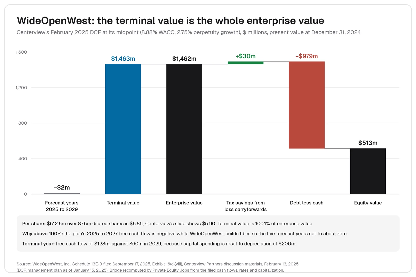
The February midpoint works the same way. The perpetuity formula gives $2,146 million at the end of 2029, or $2,239 million after the mid-year adjustment. Discounted five years at 8.88%, that is $1,463 million, against $1,462 million of enterprise value. Recomputed from the rounded cash flows on the slides, both grids match Centerview's figures to within 6 cents a share, 0.1 turn of multiple and 0.1 point of growth. Centerview's August range was $3.05 to $6.75 a share, against $3.40 to $9.30 in February, and the agreed price of $5.20 sat inside the August range.
How much of a DCF is terminal value
The terminal value's share of a DCF is its present value divided by enterprise value. The share rises when the forecast is short, when growth or the exit multiple is high, when the discount rate is low, and when the forecast years are spent investing rather than generating cash. For the steady company growing 3% a year at a 9% discount rate, it is 75% with a five-year forecast and 57% with a ten-year one. For a company in a heavy build phase, or a startup that burns cash for years, it can approach or pass 100%.
At WideOpenWest the share was 100.0% to 100.2% in the February grid and 100.2% to 100.4% in the August grid. A share above 100% is not an error. It means the cash flows in the forecast years are negative in total, so the investor pays for the whole company with cash that arrives after 2029. The entire valuation then rests on the terminal year, and the forecast matters mainly for how it gets the business there: the level of 2029 EBITDA and the drop in capital spending.
Debt magnifies terminal value assumptions for shareholders. Equity value is enterprise value minus net debt, and WideOpenWest's net debt was about two-thirds of its February enterprise value. Moving perpetuity growth from 2.5% to 3.0% at the 8.88% WACC raised the terminal value and the enterprise value by 9%, but it raised the value per share by 28%, from $5.16 to $6.61 in the recomputed grid. The same arithmetic applies to any leveraged company and to the equity in a leveraged buyout.
Because so much rests on the terminal value, a reviewer of a DCF usually reads the terminal year first: what free cash flow it assumes, how it compares with the last forecast year, and what growth rate or multiple it implies. Extending the forecast until the company has reached a steady state reduces the share without changing the answer, if the extra years are modeled consistently, but it makes the assumptions visible year by year.
Terminal value in private equity and leveraged buyouts
A leveraged buyout (LBO) model has a terminal value too, though it is rarely called that. The sponsor projects the company for the holding period, usually three to seven years, and assumes a sale at the end at a multiple of exit-year EBITDA. That exit value is an exit multiple terminal value. It is not discounted at a WACC. Instead, the equity left after repaying debt is compared with the equity invested to give the fund's internal rate of return (IRR) and multiple of money.
The same disciplines apply. The exit multiple should be one a buyer would pay for the business as it will be at exit, which is often slower-growing than at entry. Investment committees commonly ask to see a base case that exits at or below the entry multiple, so that the return comes from earnings growth and debt paydown rather than from a higher price for the same earnings. Because buyout equity is only part of enterprise value, a half turn on the exit multiple changes the equity at exit by a larger percentage than it changes enterprise value, the same leverage effect as in the WideOpenWest grid. Modeling tests for private equity interviews, such as the LBO modeling test, often ask candidates to explain or sensitize this assumption.
In WideOpenWest's case the buyers paid about 5.1 times next-twelve-month adjusted EBITDA, according to Centerview's August materials, and Centerview's terminal multiples of 5.0 to 6.0 times sat around that figure, although they were applied to terminal-year 2029 EBITDA after stock-based compensation. The buyers' own model, including their exit assumption, is not public. Take-privates that involve an affiliate, like this one, are a useful source for anyone learning valuation, because the Schedule 13E-3 usually includes the special committee adviser's full discussion materials, with the projections, discount rates and terminal assumptions that a proxy summary leaves out.
Common terminal value mistakes
- A final year that is not a steady state. Revenue still growing at 10%, margins still expanding or capital spending far from depreciation all get repeated forever. Add a normalized terminal year if the last forecast year is not representative.
- Growth with no reinvestment. A terminal year with capital spending equal to depreciation and positive growth assumes the growth costs nothing. Check it with the value-driver formula.
- A growth rate above the risk-free rate, or a nominal growth rate paired with a real discount rate, or cash flows in one currency with a discount rate from another.
- Timing errors. Using FCF(n) instead of FCF(n) × (1 + g) in the numerator, applying a forward multiple to final-year EBITDA, discounting the terminal value over n + 1 years, or using the mid-year convention for the forecast without adjusting a perpetuity growth terminal value.
- A partial final year. In a quarterly or monthly model, the terminal value has to be based on the full final year, not the last quarter or month.
- The wrong multiple. Today's multiple for fast-growing peers, a deal multiple with a control premium in a standalone valuation, or a multiple measured on a different EBITDA definition from the one it is applied to.
- The wrong formula for the metric. The perpetuity growth formula applies to after-tax free cash flow, never to EBITDA or a pre-tax figure, and unlevered cash flow goes with the WACC, levered cash flow with the cost of equity.
- Averaging the two methods instead of reconciling them through the implied growth rate and multiple.
- No cross-check at all. A model that shows a terminal value without its implied multiple, implied growth rate and share of enterprise value leaves the most important assumption unexamined.
- A perpetuity for a business with a finite life, such as a single-asset project, a key-person firm or a fund. Use a salvage or liquidation value instead.
Terminal value interview questions
Terminal value comes up in almost every DCF discussion in banking and private equity interviews. The first question is usually the definition, and the follow-ups test whether a candidate understands the assumptions.
- How do you calculate terminal value? Two ways. With the perpetuity growth method, take final-year free cash flow, grow it one year at the long-run rate and divide by WACC minus that rate. With the exit multiple method, multiply final-year EBITDA by a multiple from comparable companies or deals. Either way, discount the result to today with the final year's discount factor.
- Which method gives a higher value? Neither by nature. The answer depends on the inputs, and the two match when the growth rate equals the one the multiple implies.
- What growth rate would you use? A long-run nominal rate below the growth of the economy and below the risk-free rate, typically 2% to 3% for a mature US company. Then check what it implies as a multiple.
- How would you check an exit multiple? Back out the implied perpetuity growth rate: (terminal value × WACC − FCF) / (terminal value + FCF). If it is above the risk-free rate, the multiple is too high.
- If the WACC rises, what happens to terminal value under each method? Under perpetuity growth, the terminal value itself falls, because the WACC is in the denominator, and its present value falls further. Under the exit multiple method, the terminal value at year n is unchanged, and only its present value falls.
- Can terminal value be more than 100% of enterprise value? Yes, when the forecast years have negative cash flow in total, as at WideOpenWest in 2025, where heavy capital spending made the first three years negative.
- Why does the mid-year convention affect the terminal value? If forecast cash flows are discounted from mid-year, a perpetuity growth value has to be adjusted by (1 + WACC)^0.5 to be consistent. An exit multiple is a price at year-end and is discounted over the full n years.
- What is the terminal value in an LBO? The exit value, which is exit-year EBITDA times the exit multiple. It is not discounted at a WACC but compared with the equity invested to give the IRR.
Analyst and associate roles where DCF and LBO models are daily work are listed on Private Equity Jobs.
Terminal value FAQs
Is terminal value the same as salvage value?
They are related. Salvage value is what an asset or project is expected to be sold for at the end of its useful life, net of tax, and in capital budgeting it is the closing value of a project with a finite life. Terminal value in a DCF usually assumes the business continues indefinitely and is valued as a going concern. When a business will not continue, the terminal value should be a salvage or liquidation value.
What is the terminal value in an NPV calculation?
Net present value (NPV) is the present value of all future cash flows minus the initial investment. When the cash flows run beyond the forecast, the terminal value is added to the final year's cash flow and discounted with it, so the present value of the terminal value is one component of NPV. In project models a common error is to calculate the terminal value and forget to include it in the cash flow line before the NPV is computed.
Is perpetuity growth the same as the Gordon growth model?
Yes. The Gordon growth model values a stream of dividends that grows at a constant rate forever, D(1) / (r − g). The perpetuity growth method applies the same formula to free cash flow and the WACC.
What does a negative terminal value mean?
Either the final-year free cash flow is negative, so the business is assumed to consume cash forever, or the growth rate is at or above the discount rate, which makes the formula meaningless. The first calls for a longer forecast or a different terminal year, and the second for a lower growth rate. A business that will lose money indefinitely should be valued at its liquidation value.
How do you handle a company that may not survive to the terminal year?
A terminal value assumes the company is still operating at the end of the forecast. For a young or cash-burning company that may not get there, Damodaran's paper weights the going-concern DCF value by the probability of survival and a distressed sale value by the probability of failure. A company with a $1 billion DCF value, a $500 million distressed sale value and a 20% chance of failure is worth $1,000 million × 0.8 + $500 million × 0.2, or $900 million. The loss comes from the discount in a forced sale, not from the failure itself.
How long should the forecast be before the terminal value?
Long enough for the business to reach a steady state, which is usually five to ten years. Damodaran, in his recorded lecture, says the median high-growth period for US growth companies is about three to five years, that about 99% last less than ten, and that he never uses more than ten. He sets the length from the company's size relative to its market, its recent revenue growth and how durable its competitive advantages are. A forecast that ends too early puts more of the value into the terminal value and makes the terminal year less reliable. A forecast that runs for decades assumes excess returns that competition usually removes sooner.
How do you calculate terminal value in Excel?
Put the final-year free cash flow, the growth rate and the WACC in separate cells and enter =FCF(1+g)/(WACC-g) for the perpetuity growth method, or =EBITDAmultiple for the exit multiple method. Discount with =TV/(1+WACC)^n, or with the XNPV function if the cash flows have specific dates. Build a data table to show the value across a grid of discount rates and growth rates or multiples.
Sources
WideOpenWest, Inc., Schedule 13E-3 filed September 17, 2025: Exhibit 16(c)(viii), Centerview Partners discussion materials, February 13, 2025 (Management Plan Summary; Discounted Cash Flow Analysis; Net Operating Losses), Exhibit 16(c)(x), Centerview discussion materials, May 30, 2025, and Exhibit 16(c)(xii), Centerview discussion materials, August 10, 2025 (Discounted Cash Flow Analysis; Multiple Evolution Over Time; Selected Precedent Transactions); definitive proxy statement (DEFM14A), filed October 27, 2025: Opinion of Centerview Partners LLC. Aswath Damodaran, NYU Stern, "Closure in Valuation: Estimating Terminal Value". Aswath Damodaran, "Session 9: Terminal Value", recorded lecture, August 2014. The Footnotes Analyst, "DCF terminal values: Using the right exit multiple" and "DCF terminal values: Returns, growth and intangibles", October 2021. US Department of the Treasury, Daily Treasury Par Yield Curve Rates, 2026 and 2025.
Related posts
Related posts
Valuation methods explained: the income, market and asset approaches, the methods bankers and private equity firms use, how to choose one, and Clearwater Analytics' $24.55 take-private valued by two banks with every method.
WACC is the blended return a company owes its lenders and shareholders. The formula, each input with 2026 data, and two banks' filed WACCs for the same company in the same week, rebuilt line by line.
A discounted cash flow analysis values a business at what its future cash is worth today. The formula, the six steps, WACC and terminal value, and a filed 2026 take-private DCF rebuilt line by line.