
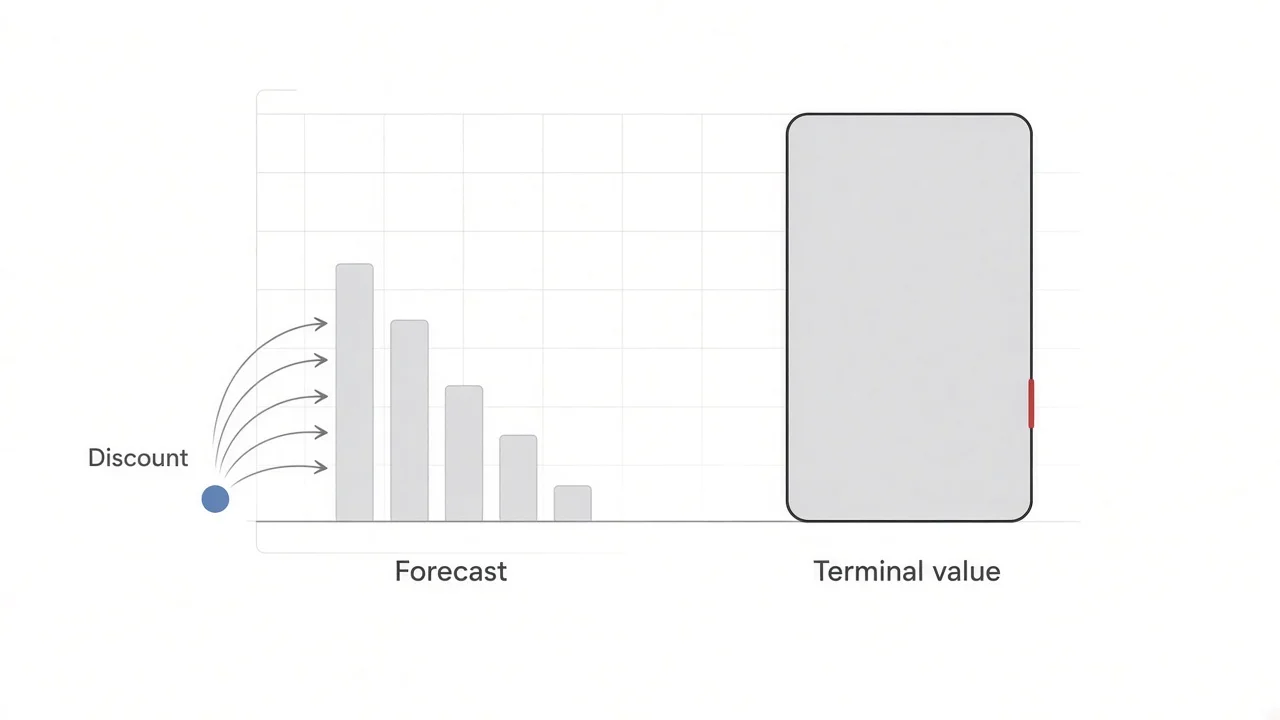
A discounted cash flow (DCF) analysis values a business at what its future cash is worth today. An analyst forecasts the cash the company will generate for its lenders and shareholders over the next five to ten years, estimates a single terminal value for all the years after that, and discounts both back to the present at a rate that reflects the risk of the business, usually the weighted average cost of capital (WACC). The total is the value of the whole company; subtracting net debt and dividing by the share count gives a value per share. In July 2026, when a special committee of Distribution Solutions Group's board weighed a $35-a-share offer from LKCM Headwater, the private equity firm that already controlled the company, its banker, William Blair, ran management's five-year forecast through a DCF at discount rates of 9% to 11% and long-term growth of 2% to 3%. The answer was $24.86 to $42.63 a share. Rebuilt from the same filing, about three-quarters of that value sits in the terminal value, and from the midpoint a one-point change in the discount rate moves the result by $5.61 to $7.35 a share. A handful of inputs decide almost the whole answer, which is why bankers present a DCF as a range and why buyers and sellers argue about the assumptions rather than the arithmetic.
What a discounted cash flow analysis is
A DCF rests on one idea: a business is worth the cash it will produce over its life, adjusted for when that cash arrives and how likely it is to arrive. A dollar received in five years is worth less than a dollar today, because today's dollar could be invested in the meantime and because the future dollar might not show up. Discounting turns each future dollar into its present value at a rate that pays an investor for both the wait and the risk.
That makes a DCF an intrinsic valuation. It estimates value from the company's own forecast, without reference to what investors are paying for other companies. Comparable company analysis and precedent transactions work the other way: they read prices off similar companies and deals and carry them across. Warren Buffett's definition of intrinsic value in Berkshire Hathaway's owner's manual is a DCF in one sentence: "the discounted value of the cash that can be taken out of a business during its remaining life." For a listed company, a DCF value above the share price suggests the stock is undervalued on the analyst's assumptions, and a value below it suggests the stock is overvalued. Because the answer is a range, investors usually want a wide gap, a margin of safety, before acting on it.
The cash in question is free cash flow, not accounting earnings. Net income includes non-cash charges such as depreciation, records sales before customers pay, and ignores the money spent on new equipment and inventory. Free cash flow is what is left after the business has paid its operating costs and taxes and funded the investment it needs to keep growing.
Most company DCFs value the whole enterprise. They forecast unlevered free cash flow, the cash available to all providers of capital before any interest or debt repayment, and discount it at the WACC, a blend of what lenders and shareholders require. The result is enterprise value, which is then split between debt and equity. A levered DCF instead forecasts the cash left for shareholders after debt service and discounts it at the cost of equity alone, arriving at equity value directly. In theory the two agree. In practice bankers and buyout investors use the unlevered version, because it does not depend on a capital structure that is about to change in a sale or a leveraged buyout (LBO).
Because no one can forecast a company year by year forever, a DCF has two stages. The first is an explicit forecast, typically five years for a mature company and ten or more for one that is still growing fast. The second is a terminal value, a single number that stands in for every year after the forecast, calculated either by assuming cash flow grows at a steady rate forever or by assuming the business is sold at a multiple of its earnings. A single asset such as a machine or a building is valued over its useful life instead, with any resale value at the end in place of a terminal value.
Investment bankers build DCFs for fairness opinions and pitch books, equity research analysts use them to set price targets, and corporate finance teams use the same arithmetic to decide whether a new plant earns more than its cost of capital, or more than a higher hurdle rate when the project is riskier than the company as a whole.
The DCF formula
Each future cash flow is divided by one plus the discount rate, raised to the number of years until the cash arrives:
Present value = CF₁ / (1 + r)¹ + CF₂ / (1 + r)² + ... + CFₙ / (1 + r)ⁿ + TVₙ / (1 + r)ⁿ
CF is the cash flow in each year, r is the discount rate, n is the final year of the forecast, and TV is the terminal value at the end of year n. The terminal value is discounted with the final year's factor because it is a value as of that date.
A three-year example shows the mechanics. A business expected to generate $100 next year, $110 the year after and $121 in year three, discounted at 10%, has explicit cash flows worth $90.91 each today, $272.73 in total, because the growth exactly offsets the discount each year. If cash flow then grows at 3% a year forever, the terminal value at the end of year three is $121 × 1.03 / (10% − 3%) = $1,780.43, worth $1,337.66 today. The business is worth $1,610.39, and 83% of that comes from the years after the forecast.
A DCF and net present value (NPV) use the same discounting. NPV then subtracts the upfront cost of the investment. If the business above could be bought for $1,400, the NPV of buying it at a 10% required return would be $210.39. The same idea runs in reverse: paying less than the DCF value means earning more than the discount rate, and paying more means earning less. The rate that makes the NPV exactly zero is the internal rate of return, the measure private equity firms use to price deals.
In Excel, =NPV(rate, cash flows) assumes each cash flow arrives at the end of evenly spaced periods. =XNPV(rate, cash flows, dates) discounts each flow to its actual date, which matters when a deal closes partway through a year.
How to build a DCF model, step by step
A DCF model has six steps:
- Forecast unlevered free cash flow for five to ten years.
- Calculate the discount rate, the weighted average cost of capital.
- Calculate the terminal value at the end of the forecast.
- Discount the cash flows and the terminal value to the valuation date.
- Move from enterprise value to equity value per share.
- Run sensitivity tables and scenarios.
1. Forecast unlevered free cash flow
Unlevered free cash flow starts from operating profit and strips out everything to do with financing:
Unlevered free cash flow = earnings before interest and taxes (EBIT) × (1 − tax rate) + depreciation and amortization − capital expenditures − increase in net working capital
EBIT is the operating profit line. Taxing it at the company's rate gives net operating profit after tax (NOPAT), the tax the business would pay if it had no debt. Depreciation and amortization are added back because they reduce profit without using cash. Capital expenditures are subtracted because they use cash without reducing profit. An increase in net working capital (receivables plus inventory minus payables) is cash tied up in the business, so it is subtracted; a decrease releases cash. Interest expense, interest income, dividends and debt repayments stay out, because the discount rate already accounts for what lenders and shareholders are owed.
The forecast is the hard part. Revenue is projected as a growth rate for a stable company or built from drivers such as units and prices or customers and revenue per customer. Margins come from the company's history, its plans and its peers. Capital expenditures should run ahead of depreciation while the company is growing, and working capital usually follows revenue, either as a percentage of sales or as days of receivables, inventory and payables. The cleanest models drive all of this from a linked three-statement model. Inputs come from annual and quarterly filings, investor presentations, industry research, management guidance and, in a sale, management's own projections, which a proxy statement prints.
Three items cause most disagreements. Stock-based compensation is a real cost paid in shares rather than cash, and adding it back overstates free cash flow while the share count quietly grows. Distribution Solutions Group's projections add it back to reach adjusted earnings before interest, taxes, depreciation and amortization (EBITDA) and then subtract it again before computing unlevered free cash flow, and Citi's DCF of the software company Jamf, in a proxy statement filed in December 2025 for its sale to Francisco Partners, states that stock-based compensation "was treated as a cash expense." Leases are the second: under US accounting, operating lease rent stays in operating costs and should stay there, while under the international lease standard, IFRS 16, part of the rent is booked as interest and depreciation, which inflates EBITDA unless the analyst deducts the full lease cost or counts lease liabilities as debt, but not both. One-time items are the third: restructuring charges and acquisition costs are excluded from the run rate only if they really will not recur.
2. Calculate the weighted average cost of capital
Unlevered free cash flow belongs to lenders and shareholders together, so it is discounted at their blended required return:
WACC = E / (D + E) × cost of equity + D / (D + E) × cost of debt × (1 − tax rate)
E and D are the market values of equity and debt, or a target mix when the current one is expected to change. The cost of debt is the yield the company would pay to borrow today, not the coupon on old bonds, and it is reduced by the tax rate because interest is deductible. The cost of equity cannot be observed, so it is estimated with the capital asset pricing model (CAPM):
Cost of equity = risk-free rate + beta × equity risk premium
The risk-free rate is usually the 10-year US Treasury yield. The equity risk premium is the extra return investors expect from stocks over that bond. Beta measures how much the stock moves with the market; a beta of 1.2 means the stock tends to rise or fall 12% when the market moves 10%. Because beta reflects past share-price swings rather than business risk, some analysts replace it with a premium built from the business itself: how cyclical it is, its size, the strength of its balance sheet and how durable its competitive position is. Because the risk-free rate moves with inflation and interest rates, the same forecast is worth less when Treasury yields rise.
Aswath Damodaran of NYU Stern publishes these inputs every January. His US cost of capital data for January 2026 puts the 62 listed companies in his distributors industry group at a beta of 0.95, and his implied equity risk premium series starts 2026 with a 10-year Treasury yield of 4.18% and a premium of 4.23%. The cost of equity is therefore about 4.18% + 0.95 × 4.23% = 8.2%. With a pre-tax cost of debt of 5.07%, an effective tax rate of 14.59% and debt at 22% of capital, the industry WACC works out to 0.78 × 8.18% + 0.22 × 3.80% = 7.22%.
William Blair used 9% to 11% for Distribution Solutions Group, a premium of roughly two to four points over that industry figure. The filing says only that the range reflected "professional judgment" and a CAPM-based WACC. A company with an equity value of about $1.6bn at the offer price and net debt of roughly four times EBITDA carries more risk than the industry average, and many bankers add a size premium for smaller companies. Software sits higher still: Citi discounted Jamf at 12.1% to 13.5%. When a company is private and has no beta, analysts take the betas of listed peers, remove the effect of each peer's debt (unlevering), average them, and add back the target's own leverage (relevering).
3. Calculate the terminal value
The perpetuity growth method, also called the Gordon growth method, assumes free cash flow grows at a constant rate forever after the final forecast year:
Terminal value = final-year free cash flow × (1 + g) / (WACC − g)
The growth rate g has to be low, at or below long-run nominal growth in the economy, usually 2% to 3% for a US company, because no business can outgrow the economy forever. The formula also explodes as g approaches the WACC: at 3% growth, cutting the discount rate from 10% to 9% raises the terminal value by 16.7%.
The exit multiple method assumes the business is sold at the end of the forecast at a multiple of its final-year earnings, usually the ratio of enterprise value to EBITDA paid for comparable companies or in recent deals:
Terminal value = final-year EBITDA × exit multiple
Bankers and private equity investors often prefer the exit multiple because it matches how deals are priced. Its weakness is that it imports today's market prices into a method meant to be independent of them, and it is easy to pick a multiple that implies a growth rate no company could sustain. Many practitioners therefore start with the growth rate and check the multiple it implies. The two methods check each other. A perpetuity terminal value divided by final-year EBITDA gives the implied exit multiple; an exit-multiple terminal value can be solved for the growth rate it implies with g = (TV × WACC − FCF) / (TV + FCF), where FCF is final-year free cash flow. If one method implies 6% growth or the other a multiple far from where peers trade, the assumption needs work.
The final forecast year has to be a steady state before either method is applied. Margins should have stopped expanding, capital spending should be close to what maintenance and modest growth require, and cash flow growth should be near the terminal rate. If cash flow is still growing 12% in the last forecast year and drops to 2% in the terminal value, the forecast is too short or the terminal rate too low.
4. Discount the cash flows to the valuation date
Each cash flow is multiplied by a discount factor of 1 / (1 + WACC)ᵗ, where t is the time in years from the valuation date. Two timing choices change the answer by a few percent.
The first is the stub period. If the valuation date is March 31 and the forecast runs on calendar years, only the last nine months of the current year's cash flow belong to the buyer, so the first year is cut to 75% and every later year is discounted from March 31. The second is the mid-year convention. Cash arrives through the year, not on December 31, so many bankers discount each year's flow from the middle of its period (t = 0.5, 1.5, 2.5 and so on, adjusted for the stub). That raises value by roughly half a year of discounting. The terminal value is usually discounted from the end of the final year under the exit multiple method, because a sale happens at a point in time; under the perpetuity method practitioners differ. On the Distribution Solutions Group figures, switching from year-end to mid-year discounting adds 1.7% to the value per share.
The sum of the discounted cash flows and the discounted terminal value is enterprise value.
5. Move from enterprise value to equity value per share
Enterprise value belongs to everyone with a claim on the business. To find what belongs to common shareholders, subtract every claim that ranks ahead of them and add assets the cash flow forecast left out:
- Subtract total debt, including the current portion, and finance leases (and operating leases if lease costs were added back in the forecast).
- Subtract preferred stock and non-controlling interests, the share of consolidated subsidiaries owned by outsiders.
- Add cash and marketable securities, equity stakes and other non-operating assets.
- Add the present value of tax losses that will reduce future taxes, if the forecast did not use them. William Blair added the present value of the tax savings from $4m of Distribution Solutions Group's federal net operating losses.
Net debt is debt and other claims minus cash and non-operating assets. Equity value is enterprise value minus net debt, and value per share is equity value divided by diluted shares: basic shares plus restricted stock units and in-the-money options and convertibles, with options counted by the treasury stock method (only the shares left after the exercise proceeds buy some back). Because which options are in the money depends on the share price the DCF is solving for, the share count and the price are usually calculated together. William Blair counted Distribution Solutions Group's options at a weighted average strike of $42.29 and left out the tranches that were out of the money.
6. Run sensitivity tables and scenarios
A DCF is presented as a range, never a point. The standard output is a two-way table that recalculates value per share across a grid of discount rates and terminal growth rates (or exit multiples), built with Excel's data table function. Analysts add operating scenarios as well, because the forecast drives the answer as much as the rates: a base case, a downside case with slower growth or thinner margins, and sometimes an upside case. Distribution Solutions Group's special committee asked William Blair to run a "sensitivity case" with lower margin expansion and greater execution risk; it produced a lower range, which the filing describes but does not quantify. The DCF range then sits on a football field chart beside the ranges from comparable companies, precedent transactions and a buyout analysis, with the offer price drawn across all of them.
DCF example: Distribution Solutions Group's 2026 take-private
Distribution Solutions Group is a Fort Worth, Texas, specialty distributor of industrial supplies, the parent of Lawson Products, Gexpro Services and TestEquity. LKCM Headwater and its affiliates owned about 78.5% of the stock when LKCM Headwater proposed to buy the rest for $29.50 a share in March 2026. A special committee of independent directors negotiated the price up through $31.00, $32.75 and $34.00 to $35.00, with William Blair presenting a preliminary DCF at most rounds, and signed a merger agreement on July 15, 2026. The company's definitive proxy statement, filed with the SEC on October 28, 2026, prints management's projections and the inputs of William Blair's DCF, which makes it possible to rebuild the analysis. The stockholder vote is scheduled for November 27, 2026.
The projections
Management's revised projections, approved by the special committee on July 8, 2026 for William Blair's use, assume revenue growth of 6% to 7% a year and about 3.9 percentage points of margin expansion. The unlevered free cash flow build follows the formula in step 1 ($m):
| 2025 pro forma | 2026 | 2027 | 2028 | 2029 | 2030 | |
|---|---|---|---|---|---|---|
| Revenue | 1,989 | 2,150 | 2,256 | 2,414 | 2,574 | 2,746 |
| Adjusted EBITDA | 178 | 203 | 232 | 277 | 313 | 352 |
| Less stock-based compensation and other adjustments | (16) | (13) | (12) | (12) | (12) | (12) |
| EBITDA | 162 | 190 | 220 | 265 | 301 | 340 |
| Less depreciation and amortization | (81) | (82) | (77) | (73) | (70) | (60) |
| EBIT | 81 | 108 | 143 | 192 | 231 | 280 |
| Less taxes at 29.5% | (24) | (32) | (42) | (57) | (68) | (83) |
| NOPAT | 57 | 76 | 101 | 135 | 163 | 197 |
| Plus depreciation and amortization | 81 | 82 | 77 | 73 | 70 | 60 |
| Less capital expenditures | (27) | (28) | (26) | (28) | (30) | (32) |
| Less increase in net working capital | (2) | (67) | (10) | (24) | (38) | (41) |
| Unlevered free cash flow | 109 | 63 | 142 | 157 | 166 | 186 |
Two lines stand out. Working capital absorbs $67m in 2026, against $27m in management's April projections, which cuts that year's free cash flow from $106m to $63m. And depreciation and amortization falls from $82m to $60m while capital spending rises, so by 2030 the business converts 55% of its EBITDA into unlevered free cash flow.
William Blair's assumptions
The filing lists every input except the valuation date:
- Cash flows: unlevered free cash flow for 2026 through 2030, after tax at 29.5%.
- Discount rate: 9.0% to 11.0%, from a CAPM-based WACC and professional judgment.
- Terminal value: perpetuity growth of 2.0% to 3.0% applied to 2030 free cash flow.
- Tax assets: the present value of tax savings from $4m of federal net operating losses.
- Net debt: $685m as of March 31, 2026.
- Shares: 46,255,422 common shares, 424,717 restricted stock units, 115,988 deferred shares and the in-the-money portion of 2,258,658 options (weighted average strike $42.29).
The result: $24.86 to $42.63 a share, against the $35.00 offer.
Rebuilding the range
Private Equity Jobs rebuilt the analysis with three assumptions the filing does not state for the final run: a March 31, 2026 valuation date (the date William Blair's preliminary DCF used), the mid-year convention, and nine months of 2026 cash flow. The share count is 46.80m, the listed shares and units without the option tranches, which the filing does not itemize.
| Low (11% WACC, 2% growth) | Middle (10%, 2.5%) | High (9%, 3%) | |
|---|---|---|---|
| Present value of 2026 to 2030 cash flows ($m) | 532 | 544 | 557 |
| Terminal value at end of 2030 ($m) | 2,108 | 2,542 | 3,193 |
| Present value of terminal value ($m) | 1,284 | 1,616 | 2,120 |
| Enterprise value, including tax losses ($m) | 1,817 | 2,161 | 2,678 |
| Less net debt ($m) | (685) | (685) | (685) |
| Equity value ($m) | 1,132 | 1,476 | 1,993 |
| Value per share | $24.18 | $31.55 | $42.59 |
| Terminal value share of enterprise value | 71% | 75% | 79% |
| Terminal value / 2030 adjusted EBITDA | 6.0x | 7.2x | 9.1x |
The rebuild lands at $24.18 to $42.59, within 4 cents of the filed top and 68 cents below the filed bottom; the likely gaps are the exact valuation date and the options.
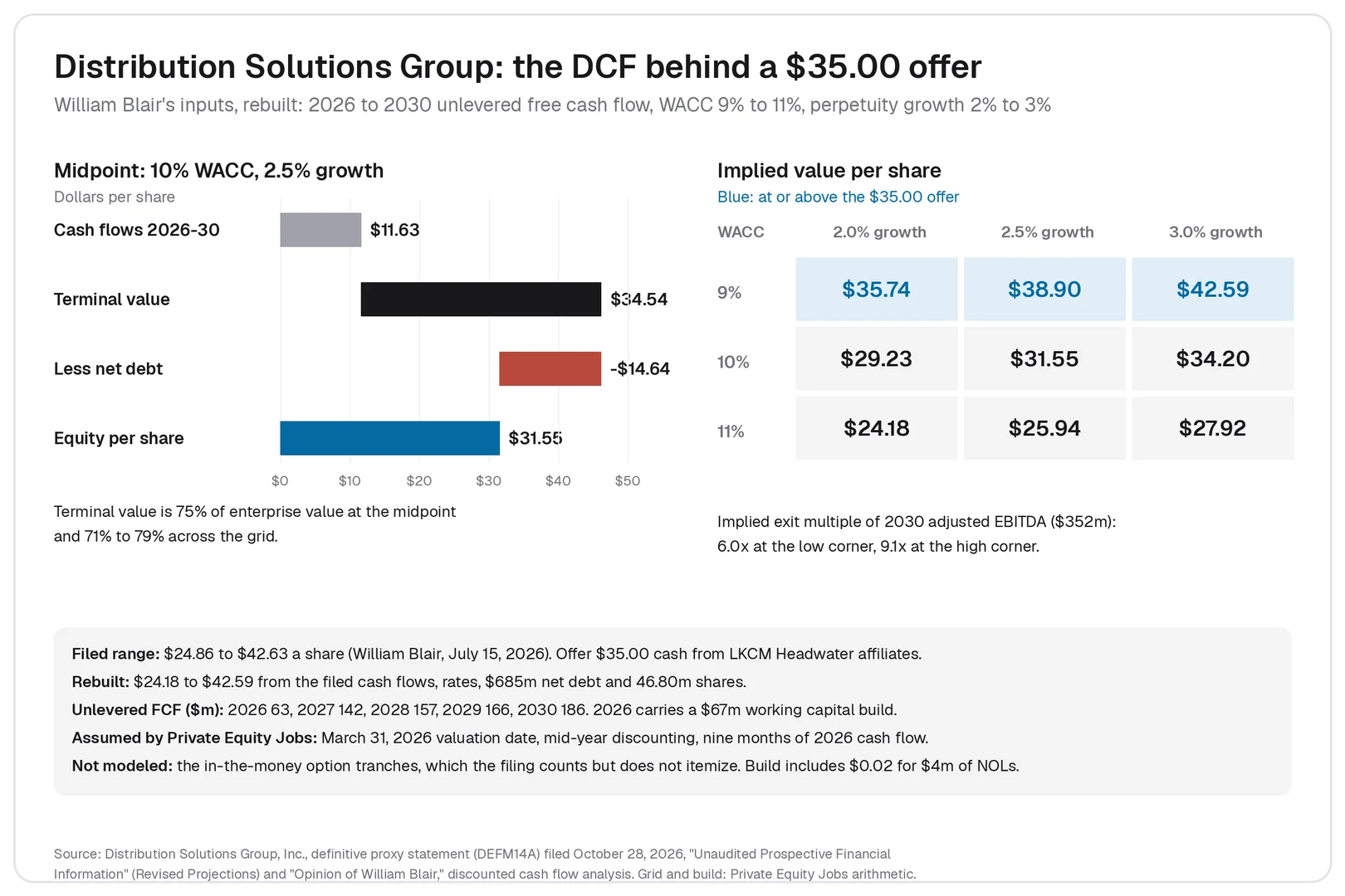
Only the 9% row clears $35.00 at every growth rate; at 10% the value runs from $29.23 to $34.20, and at 11% from $24.18 to $27.92.
| WACC | 2.0% growth | 2.5% growth | 3.0% growth |
|---|---|---|---|
| 9.0% | $35.74 | $38.90 | $42.59 |
| 10.0% | $29.23 | $31.55 | $34.20 |
| 11.0% | $24.18 | $25.94 | $27.92 |
What the DCF says about the $35.00 price
The terminal value carries 71% to 79% of the enterprise value, so the debate over the price is mostly a debate over what the business is worth after 2030. The implied exit multiples, 6.0x to 9.1x 2030 adjusted EBITDA of $352m, are low next to the 15.8x median trailing multiple of the seven listed distributors William Blair compared, and mostly below the 9.0x to 11.0x exit range it used in its own buyout analysis of the same company. Solving the other way, a 9x to 11x exit on $352m at a 9% discount rate implies perpetual growth of 3.0% to 4.0%; at 11%, 4.8% to 5.9%. The perpetuity method with 2% to 3% growth is the more conservative of the two.
The forecast also ends while growth is still high. Free cash flow rises 12.0% in 2030, from $166m to $186m, then grows 2% to 3% a year in the terminal value. That step-down lowers value; a longer forecast that let growth fade would raise it. A seller could argue the range understates the business for that reason; a buyer could answer that the margin expansion behind the forecast is not yet earned. The offer of $35.00 sits inside the filed range, above its midpoint, at 11.5 times management's 2026 adjusted EBITDA of $203m.
DCF vs comparable company analysis and precedent transactions
The three methods answer different questions. A DCF asks what the cash flows are worth at a chosen required return, so its answer moves with the forecast and the rates. Comparable company analysis asks what the stock market is paying today for similar businesses, per dollar of EBITDA or earnings; it needs no forecast beyond a year or two, but it inherits whatever the market is getting wrong. Precedent transactions ask what buyers have paid for whole companies, which includes a premium for control and reflects the credit markets of the years when those deals closed.
A DCF leads when a company has predictable cash flows and few true peers; multiples lead when the forecast is unreliable. Bankers show all three on a football field. For Distribution Solutions Group, the $35.00 offer equaled 13.5 times trailing adjusted EBITDA, against a 15.8x median for listed peers and an 11.3x median for 12 selected acquisitions. An exit-multiple terminal value borrows from the other two methods, and a sum-of-the-parts valuation often runs a separate DCF for each segment.
How private equity firms use a DCF
A leveraged buyout model is a DCF turned around. A DCF fixes the discount rate and solves for value. A buyout model fixes the return the fund wants, usually an internal rate of return of 20% or more for equity, assumes an exit multiple and a debt package, and solves for the highest entry price the cash flows can support after interest and debt repayment.
William Blair ran both on Distribution Solutions Group. Its buyout analysis assumed net debt of $920m, about 5.3 times trailing adjusted EBITDA, an exit at 9.0x to 11.0x 2030 adjusted EBITDA of $357m, and target returns of 18% to 22%, and produced $26.61 to $37.00 a share. The DCF, at a 9% to 11% WACC, produced $24.86 to $42.63. The buyout range is narrower because the exit multiple anchors it, and its top end shows what a financial buyer targeting an 18% return could pay on management's plan.
A fund's equity, levered five times, needs to earn far more than the company's WACC, so a price that is fair on a DCF can still fail the fund's return test. That is why buyout investors lean on the buyout model and on multiples.
Private equity firms still build DCFs, for four purposes:
- To test the exit multiple. If a buyout model assumes a sale at 11x, a DCF shows the perpetual growth that multiple implies, as in the 3.0% to 5.9% range above.
- To value long-dated, contracted cash flows such as infrastructure and royalties.
- To value minority and growth investments, where the fund cannot add leverage or control the exit.
- To value portfolio companies at fair value for quarterly reports to investors, where the fair value accounting standard (ASC 820 in the US) allows an income approach beside the market approach.
In diligence the fund builds its own forecast, the sponsor case, usually below management's. A proxy statement DCF uses management's case, because the board's question is whether the price is fair to selling shareholders.
Valuing a private company or startup with a DCF
The mechanics are the same for a private company; the inputs are harder. There is no market beta, so analysts borrow and relever the betas of listed peers, and many add premiums for small size and for shares that cannot be sold easily. The forecast often starts from financial statements that mix the owner's personal costs with the business's, so earnings are first adjusted to a normal level, the work a quality of earnings review does in a sale.
Startups are harder still. Cash flow is negative for years, so nearly all the value sits in the terminal value, and the forecast has to run long enough for the company to reach a stable margin. EY's 2019 guide to startup valuation for founders recommends a discount rate above 25% for an early-stage company, against the 5% to 8% typical of large, stable corporations, and a worst, base and best case forecast. Venture investors more often price rounds on revenue multiples and target ownership, and treat a startup DCF as a consistency check on the plan.
Strengths and limits of a DCF
A DCF values a business on its own cash flows, so it works when there are no good peers or when the market is mispricing a whole sector. It puts every assumption in the open, so two people who disagree can see exactly where, and it ties value to decisions management controls, such as working capital and capital spending.
The limits follow from the same features. The answer is only as good as a forecast that runs five or more years out, and most of the value sits in a terminal value that rests on two numbers. Raising the discount rate by one point cut the Distribution Solutions Group value by 17% to 20%. A DCF is a poor fit for companies with negative or erratic cash flow and for banks and insurers, whose debt is raw material rather than financing; those are valued on equity cash flows or dividends instead.
Common DCF mistakes
- Mixing cash flows and rates: discounting unlevered cash flow at the cost of equity, or levered cash flow at the WACC.
- A terminal growth rate above long-run economic growth, or close enough to the WACC that the terminal value balloons.
- A forecast that ends mid-growth, with cash flow growing 10% or more in the final year and 2% in the terminal value.
- Adding back stock-based compensation and then valuing the shares it will create as if they did not exist.
- Getting the working capital sign wrong: an increase is a use of cash.
- Mixing nominal and real figures: cash flows forecast in today's dollars discounted at a rate that includes expected inflation, or the reverse.
- Using basic shares, or a share count that ignores in-the-money options at the price the DCF produces.
- Leaving out debt-like items in the bridge, such as leases, pension deficits and non-controlling interests.
- Mid-year discounting for the forecast years with an exit-multiple terminal value also discounted from mid-year.
DCF questions in interviews
"Walk me through a DCF" is the most common technical question in banking and private equity interviews. A complete answer: forecast unlevered free cash flow for five to ten years; calculate a terminal value; discount both at the WACC to get enterprise value; subtract net debt to reach equity value; divide by diluted shares. Follow-ups test whether the candidate understands the model:
- What happens if the WACC rises? Every discount factor falls and the terminal value shrinks, so value drops. On Distribution Solutions Group, moving from 10% to 11% at 2.5% growth cuts the value from $31.55 to $25.94, or 18%.
- Which matters more, one point on the discount rate or half a point on terminal growth? Usually the discount rate. In the same grid, half a point more growth adds 8% ($31.55 to $34.20).
- Why use the WACC for unlevered cash flow? Because that cash belongs to lenders and shareholders, so the rate has to reflect both of their required returns.
- How does $10 more depreciation affect value? If it is deductible for tax, operating profit falls by $10, taxes fall by $10 times the tax rate, and the $10 is added back, so free cash flow rises by the tax saving, $2.50 at a 25% rate.
- Why might a DCF and comps disagree? The DCF uses the analyst's forecast and required return; comps use the market's.
- When would you not use a DCF? For banks and insurers, and for companies with no predictable cash flow.
Buyout interviews add an LBO modeling test. Candidates who want practice usually build a first model on a mature company with simple financial statements, copying several years of figures from its annual report into a spreadsheet before forecasting. Analyst and associate roles where DCFs are routine work are listed on Private Equity Jobs, and the sponsors behind them in the companies directory.
Discounted cash flow FAQs
Is DCF the same as NPV?
They use the same discounting. A DCF sums the present values of future cash flows to estimate what an asset is worth; NPV subtracts the price or upfront cost from that sum to show whether an investment earns more than the discount rate.
Does Warren Buffett use DCF?
In principle. Berkshire Hathaway's owner's manual, issued by Buffett in June 1996, defines intrinsic value as discounted cash, adds that the calculation "is not so simple," and notes that Berkshire never gives its own estimates.
How long does it take to build a DCF model?
A quick DCF from historical figures and a few assumptions takes an experienced analyst a few hours. A full model driven by a three-statement forecast, with scenarios and sensitivity tables, takes days, and bankers refine it through a live deal as diligence improves the forecast. Outside a deal, analysts update a model when the company reports results, when guidance changes or when interest rates move.
What is a reverse DCF?
A reverse DCF starts from the current share price and solves for the growth rate or margin the price implies. It turns the question from what a company is worth into what the market already expects, which is often easier to judge.
Sources
Distribution Solutions Group, Inc., definitive proxy statement (DEFM14A), filed October 28, 2026: Unaudited Prospective Financial Information (Revised Projections), Opinion of William Blair (discounted cash flow, leveraged buyout, selected public companies and selected transactions analyses) and Summary of Discussion Materials. Jamf Holding Corp., definitive proxy statement (DEFM14A), filed December 10, 2025: Opinion of Citigroup Global Markets, discounted cash flow analysis. Aswath Damodaran, NYU Stern, Cost of Equity and Capital (US) and Historical Implied Equity Risk Premiums, January 2026. Berkshire Hathaway, An Owner's Manual. EY, Startup valuation: applying the discounted cash flow method in six easy steps (2019).
Related posts
Related posts
Comparable company analysis values a business from the multiples of similar listed companies. How to pick peers, build enterprise value, calendarize and apply the range, with a filed 2026 take-private comps table.
A quality of earnings report rebuilds a company's EBITDA, working capital, and net debt before a sale. What it checks, how it differs from an audit, what it costs, and how private equity uses it, with filed deal examples.
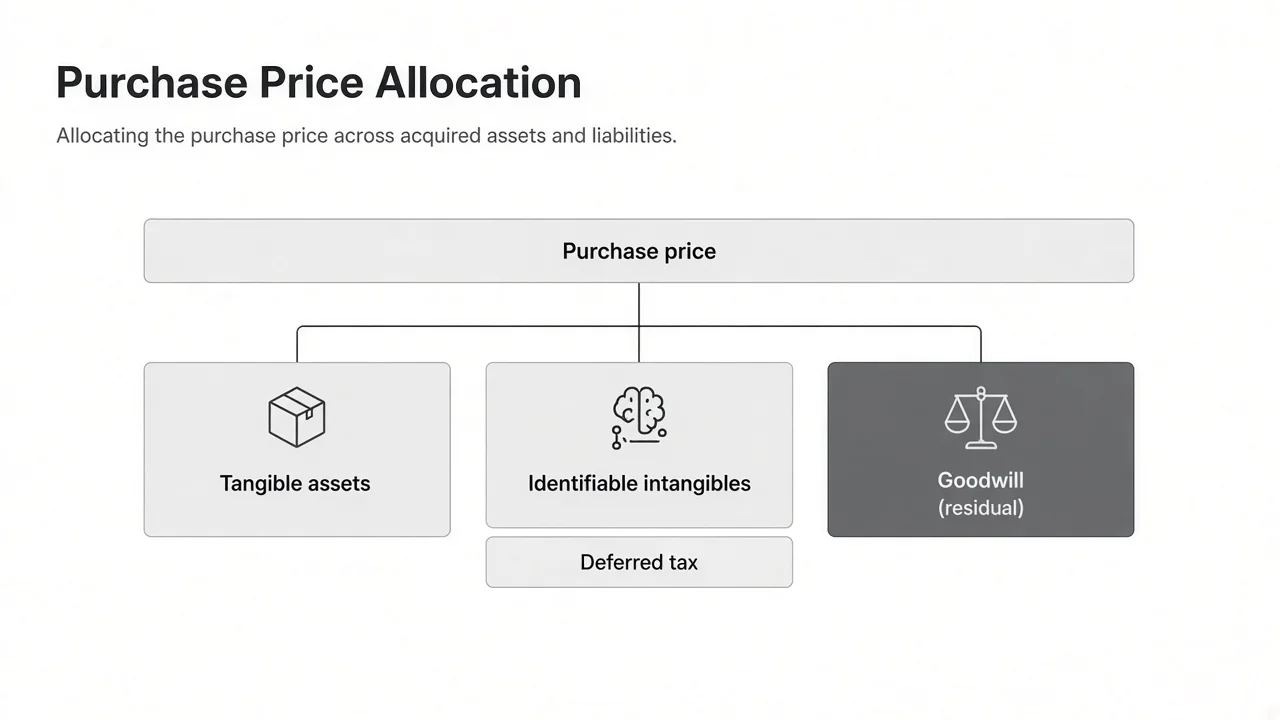
Purchase price allocation assigns a deal's price to every asset and liability at fair value and leaves goodwill as the remainder. The steps, the deferred tax math, and the tax-return version, with Kimberly-Clark's Kenvue filing.