
Comparable company analysis values a business by looking at what investors pay for similar public companies. An analyst picks a set of listed peers, divides each one's market value by a measure of its results, such as revenue or earnings before interest, taxes, depreciation and amortization (EBITDA), and applies the resulting range of multiples to the company being valued. Bankers call it trading comps, or simply comps, and it appears in nearly every pitch book, fairness opinion and private equity investment memo. In July 2026, when a special committee of Distribution Solutions Group's board weighed a $35-a-share buyout from LKCM Headwater, the private equity firm that already controlled the company, its banker compared the price with seven listed distributors trading between 8.6 and 26.8 times trailing EBITDA. The offer valued the company at 13.5 times, below the group's 15.8x median. The reasons a fair price can sit below the peer median are the substance of the method: which companies count as peers, how their numbers are made comparable, and where in the range the company belongs.
What comparable company analysis is
The premise is that companies with similar businesses, growth, margins and risks should be worth similar amounts per dollar of sales or profit. If listed industrial distributors trade at 12 to 16 times EBITDA, a private distributor with similar economics is probably worth something in that range too, adjusted for whatever makes it better or worse. The analysis does not forecast cash flows. It reads how the stock market is pricing comparable businesses today and carries that price across.
A valuation multiple has a measure of value on top and an operating figure underneath, and the two have to belong to the same group of investors. Enterprise value (EV) is the value of the whole business to lenders and shareholders together, so it is divided by figures earned before interest is paid: revenue, EBITDA, or earnings before interest and taxes (EBIT). Equity value is what belongs to shareholders alone, so it is divided by figures earned after interest: net income, or earnings per share for the price-to-earnings (P/E) ratio. An EV/EBITDA multiple of 10x means investors are paying $10 of enterprise value for every $1 of annual EBITDA.
Comparable company analysis uses share prices, which are the prices of small minority stakes traded every day. That separates it from precedent transactions, which use the prices buyers paid for whole companies, including the premium for control. Both are relative valuation methods. They tell an analyst what the market is paying, which is a price, not an estimate of what the cash flows are intrinsically worth. A multiple compresses growth, risk and cash conversion into one number, so a gap between two companies' multiples usually has a cause the analyst should find. The link to cash flow is the growing-perpetuity formula, in which value equals next year's cash flow divided by the discount rate minus the growth rate. Two companies with the same risk and the same conversion of EBITDA into cash should trade at different multiples only if the market expects them to grow at different rates.
Who uses comps and when
Investment bankers build comps for almost every assignment. They go into the valuation pages of an investment banking pitch book, into the fairness opinion a bank gives a board before it approves a sale, into the pricing of an initial public offering and follow-on stock sales, and into decisions on share buybacks. Equity research analysts keep comps tables for every company they cover and use them to set price targets. Corporate development teams and independent valuation firms use them too.
The method works best when several listed companies share the same business model, as distributors, banks and software vendors do. It works poorly for a company with no real listed peers or one that is losing money.
How to do comparable company analysis, step by step
A comps analysis has six steps. The arithmetic takes an afternoon. Most of the judgment sits in the first step and the last.
1. Select the peer group
Start with the company itself: what it sells and to whom, how fast it grows, what margins it earns, how cyclical it is and how much capital it needs. Then look for listed companies that match on those points. Industry codes help find candidates, but two companies with the same code can earn very different margins from very different customers. Candidates come from the competitors named in the annual report (Form 10-K), the pay and performance peer group in the proxy statement, equity research, fairness opinions for recent deals in the sector, and screens in services such as S&P Capital IQ.
Five to ten companies is the usual size. Fewer than five leaves the range resting on one or two names; more than ten usually means the screen let in companies that are not really comparable. Large sets are often split into tiers: closest peers by business model and size, then a wider group. Write down why each company is in or out. A missing competitor needs a reason grounded in the business, not in its multiple.
2. Gather the financial data
For each peer, collect the share price on a single date, the latest balance sheet, the share count and equity awards, historical results and consensus forecasts. Historical figures come from the latest 10-K, the quarterly reports (Form 10-Q) since then, and the earnings release filed on Form 8-K, which often arrives weeks before the 10-Q. Forecasts come from consensus estimates or research reports. Databases are faster, but filed numbers win when the two disagree. Without a paid database, the SEC's EDGAR system supplies the filings, and free sites such as Yahoo Finance list consensus estimates of revenue and earnings per share. When only an earnings per share forecast exists, a rough EBITDA estimate for the next year or two can grow last year's EBITDA at the forecast earnings growth rate. A peer listed in another currency needs its share price and its financials in the same currency, converted at the pricing date.
Every figure should be as of the same date and footnoted. Comps go stale quickly, and a table without a pricing date cannot be checked.
3. Calculate equity value and enterprise value
Equity value is the share price multiplied by fully diluted shares outstanding. Start with basic shares from the cover of the latest 10-Q, then add the shares that equity awards and convertible securities would create at today's price.
Stock options are counted with the treasury stock method. Only options with a strike price below the share price count. The method assumes holders exercise them and the company uses the cash it receives to buy back stock. With 1,000,000 options at a $20 strike and a $35 share price, exercise brings in $20m, which buys back 571,429 shares, so the net addition is 428,571 shares. Restricted stock units add one share each, because the holder pays nothing. Convertible bonds and preferred stock that are in the money are treated as converted into shares and removed from debt; if they are out of the money they stay in debt. The Distribution Solutions Group proxy lists its components: 46,255,422 common shares, 424,717 restricted stock units, 115,988 deferred shares, and 2,258,658 options with a weighted average strike of $42.29. Because that average is above the $35 offer, only the tranches with lower strikes count.
Enterprise value starts from equity value and adds every other claim on the business, less the cash a buyer would receive.
| Item | Treatment | Why |
|---|---|---|
| Equity value (diluted) | Start | Value to common shareholders |
| Total debt, including current portion and finance leases | Add | Lenders have a claim on the operating business |
| Preferred stock | Add (unless in the money and treated as converted) | A senior claim ahead of common equity |
| Noncontrolling interest | Add | EBITDA includes 100% of subsidiaries the company only partly owns |
| Cash and cash equivalents | Subtract | A buyer gets the cash and can repay debt with it |
| Equity-method investments and other non-operating assets | Subtract when material | Their earnings sit outside EBITDA |
| Operating lease liabilities, unfunded pensions | Add only if EBITDA is adjusted the same way | The numerator and denominator must match |
Citi's comps for the Jamf take-private, for example, subtracted cash and "unconsolidated assets" and added debt, preferred equity and noncontrolling interests. William Blair's definition for the Distribution Solutions Group table was equity value plus total debt, minority interest and preferred stock, less cash.
4. Spread the financials
Spreading puts every peer's revenue, EBITDA, EBIT and earnings on the same periods and definitions.
Last twelve months (LTM) figures are built from the latest annual report and the year-to-date numbers: LTM equals the last fiscal year plus the current year-to-date period minus the same period a year earlier. A company with $1,000m of revenue in fiscal 2025, $780m in the first nine months of 2026 and $740m in the first nine months of 2025 has LTM revenue of $1,040m.
Forward periods need calendarization when peers have different fiscal year-ends. A company whose year ends June 30 has half of its fiscal 2026 and half of its fiscal 2027 in calendar 2026, so calendar 2026 EBITDA equals 0.5 times fiscal 2026 plus 0.5 times fiscal 2027. A company with an August 31 year-end gets 8/12 of fiscal 2026 and 4/12 of fiscal 2027. William Blair's table footnotes both adjustments, for Applied Industrial Technologies (June) and MSC Industrial Direct (August).
Scrubbing removes items that will not recur: restructuring charges, impairments, litigation settlements, gains on asset sales, and costs tied to an acquisition. Remove them pre-tax from EBITDA and EBIT, and after tax from net income. Each company defines its own adjusted EBITDA, and the table needs one definition for everyone. Stock-based compensation is the largest inconsistency, because some companies add it back and some do not. In a software peer set, where stock pay can be a large share of revenue, that choice can move multiples by several turns. Leases are the second. Under US accounting rules, operating lease cost stays inside EBITDA; under International Financial Reporting Standards (IFRS), which most non-US companies use, almost all lease cost moves below EBITDA, which flatters an IFRS reporter's EBITDA against a US peer with the same economics.
Pro forma adjustments bring the peers up to date. If a peer closed an acquisition after its last report, add the acquired company's EBITDA and the new debt or shares that paid for it. The same applies to large buybacks, debt raises and divestitures.
5. Calculate the multiples and summary statistics
With values and metrics on the same basis, divide. Most tables show EV/Revenue, EV/EBITDA and P/E for the LTM period and one or two forward years, alongside growth, margins and leverage. A multiple built on a negative or tiny denominator is marked NM, for not meaningful, and left out of the statistics. A standard table groups each peer's market data (share price, equity value, enterprise value), its operating figures (revenue, EBITDA, growth and margins) and its multiples in separate blocks of columns, with the summary rows at the bottom.
The summary rows are the low, 25th percentile, median, mean, 75th percentile and high. The median is usually the anchor because one extreme company cannot move it. In William Blair's table, Fastenal at 26.8x pulls the mean to 16.9x while the median stays at 15.8x. A mean is reasonable only with a small set and no outliers. In a spreadsheet the summary rows are MIN, QUARTILE(range,1), MEDIAN, AVERAGE, QUARTILE(range,3) and MAX; the quartiles in the Distribution Solutions Group example below use that inclusive method.
The company being valued usually sits on its own row, outside the peer statistics, as in both fairness opinions cited here, because including it would pull the statistics toward its own current price. Comparing periods also checks the data. Multiples usually fall from the LTM column to the forward column because EBITDA is expected to grow. A forward multiple above the LTM multiple means analysts expect EBITDA to fall, as consensus did for Global Industrial (10.8x LTM, 11.3x calendar 2026).
6. Apply the range to the company
Choose a range of multiples, usually the interquartile range or a narrower band around the closest tier of peers, and place the company within it based on how its growth, margins, size and risk compare. Some analysts plot each peer's multiple against its expected growth or margin and read the company's multiple off the fitted line, which makes the placement explicit. Then work from the multiple to a price:
- Implied enterprise value equals the selected multiple times the company's metric for the same period.
- Implied equity value equals implied enterprise value minus debt, preferred stock and noncontrolling interest, plus cash.
- Implied share price equals implied equity value divided by diluted shares.
A P/E multiple skips the bridge, because it applies directly to earnings per share. Each multiple and period gives its own range, and banks show them as horizontal bars on a football field chart next to precedent transactions, a discounted cash flow analysis and, for a sponsor deal, a leveraged buyout analysis.
Which multiples to use
Enterprise value multiples are the default for most operating companies because they do not depend on how a company is financed. Two identical businesses, one funded with debt and one without, have different net income and different P/E ratios but the same EBITDA and, roughly, the same enterprise value. EV/EBITDA is also the multiple debt markets and private equity buyers use, since leveraged loans are sized as multiples of EBITDA. P/E remains standard in equity research and for sectors where debt is part of the product.
| Sector | Usual multiples | Reason |
|---|---|---|
| Industrials, distribution, consumer, business services | EV/EBITDA, EV/EBIT, P/E | Stable profits; EBIT also captures differences in capital intensity |
| Software and internet companies with thin profits | EV/Revenue, EV/gross profit, EV/free cash flow | Earnings are small or negative, or depressed by stock pay |
| Banks and insurers | P/E, price to tangible book value | Debt and deposits are the raw material, so enterprise value has no clear meaning |
| Real estate investment trusts | Price to funds from operations, implied cap rate, price to net asset value | Depreciation understates the earnings of property |
| Oil, gas and mining | EV/EBITDAX (EBITDA before exploration expense), EV per unit of reserves or production | Value rests on the resource base; exploration accounting varies |
| Retailers and restaurants | EV/EBITDA, EV/EBITDAR (EBITDA before rent) | Rent is a large cost, and adding it back puts owners and renters of stores on one basis |
The Jamf proxy shows the software case. Citi valued Jamf, which manages and secures Apple devices for businesses and which Francisco Partners agreed to buy for $13.05 a share, on calendar 2026 revenue and adjusted unlevered free cash flow rather than EBITDA. Its 18 software peers traded between 0.8x and 5.8x revenue, with a median of 2.6x. Citi applied 1.6x to 4.6x, which produced a range of $6.75 to $22.00 a share. Revenue says nothing about margins, so bankers pair a revenue multiple with a profit or cash-flow multiple.
Period matters as much as the multiple. LTM figures are real but backward-looking. Forward figures, such as the next twelve months or the next calendar year, reflect what investors are paying for, but they are forecasts. Most tables show both, and for a cyclical company the analyst has to say which year represents normal earnings.
Comparable company analysis example: a 2026 take-private
Distribution Solutions Group is a specialty distributor formed from Lawson Products, Gexpro Services and TestEquity, serving about 220,000 customers in maintenance and repair, original equipment manufacturing and industrial technology markets. LKCM Headwater, a private equity firm whose managing partner, J. Bryan King, is also the company's chief executive and chairman, owned about 78.5% of the stock together with its affiliates. On March 14, 2026, LKCM Headwater proposed to buy the rest at $29.50 a share in a going-private transaction. The board formed a special committee of independent directors, which hired William Blair as its financial advisor, and the company signed a merger agreement at $35.00 a share on July 15, 2026. The deal has not closed; the stockholder vote is scheduled for November 27, 2026. The company's definitive proxy statement, filed October 28, 2026, summarizes William Blair's analyses, including its selected public companies analysis.
The peer table
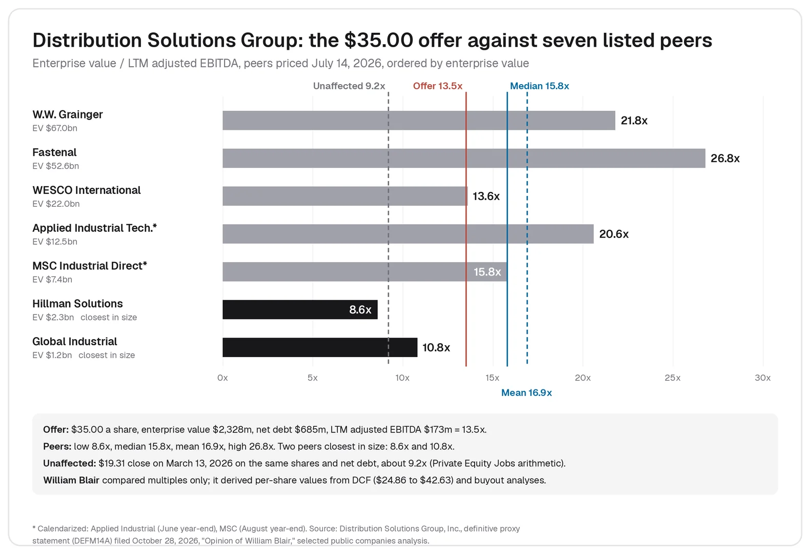
William Blair picked seven listed industrial and specialty distributors. It priced each at its July 14, 2026 close, counted diluted shares, and defined enterprise value as equity value plus total debt, minority interest and preferred stock, less cash. Multiples use LTM adjusted EBITDA and consensus estimates of calendar 2026 adjusted EBITDA.
| Company | Enterprise value ($m) | EV / LTM adj. EBITDA | EV / CY2026E adj. EBITDA |
|---|---|---|---|
| W.W. Grainger | 67,042 | 21.8x | 19.6x |
| Fastenal | 52,557 | 26.8x | 25.1x |
| WESCO International | 21,991 | 13.6x | 12.7x |
| Applied Industrial Technologies (June year-end, calendarized) | 12,451 | 20.6x | 19.4x |
| MSC Industrial Direct (August year-end, calendarized) | 7,424 | 15.8x | 14.4x |
| Hillman Solutions | 2,316 | 8.6x | 8.3x |
| Global Industrial | 1,243 | 10.8x | 11.3x |
| Low / median / mean / high | 8.6x / 15.8x / 16.9x / 26.8x | 8.3x / 14.4x / 15.8x / 25.1x | |
| Distribution Solutions Group at $35.00 | 2,328 | 13.5x | 11.5x (management) / 12.9x (consensus) |
Source: Distribution Solutions Group DEFM14A, William Blair selected public companies analysis.
At $35.00 a share, the deal implied an enterprise value of $2,328m, using net debt of $685m at March 31, 2026, against LTM adjusted EBITDA of $173m. William Blair noted that the deal multiples fell within the peer range and did not derive a per-share value from the comps. It leaned on other methods for that: a discounted cash flow analysis gave $24.86 to $42.63 a share and a leveraged buyout analysis gave $26.61 to $37.00.
Applying the range to Distribution Solutions Group
The proxy gives enough to finish the exercise. Enterprise value of $2,328m less $685m of net debt is equity value of $1,643m, or about 46.9m diluted shares at $35.00. Applying the peer statistics to LTM adjusted EBITDA of $173m gives the values below, which are Private Equity Jobs' arithmetic on the filed figures, not William Blair's.
| Multiple applied | Implied enterprise value ($m) | Implied equity value ($m) | Implied value per share |
|---|---|---|---|
| 10.8x (median of the three peers under $10bn of enterprise value) | 1,868 | 1,183 | $25.21 |
| 12.2x (25th percentile, all seven) | 2,111 | 1,426 | $30.37 |
| 13.5x (deal) | 2,328 | 1,643 | $35.00 |
| 15.8x (median, all seven) | 2,733 | 2,048 | $43.64 |
| 21.2x (75th percentile, all seven) | 3,668 | 2,983 | $63.54 |
On the full-group median, the company looks worth about $44 a share, well above the $35 price. On the 25th percentile it is worth about $30, and on the median of the three peers closest to it in size, about $25.
What the table says about the price
The peer group runs from Global Industrial, about half the enterprise value of Distribution Solutions Group, to Grainger, nearly 29 times it. Grainger and Fastenal, the two largest, trade at 21.8x and 26.8x. Hillman and Global Industrial, the two companies closest in size, trade at 8.6x and 10.8x. Placing the company within this range is the real analysis, and it points toward the lower tier. Distribution Solutions Group also carried net debt of about 4.0 times LTM EBITDA ($685m against $173m), and with affiliated holders owning 78.5% of the stock, only about a fifth of the shares traded freely. Before the first proposal, at its unaffected close of $19.31 on March 13, 2026, the company traded at roughly 9.2x LTM EBITDA on the same share count and net debt, by Private Equity Jobs' arithmetic, close to its smallest peers.
That is why a price below the peer median could still be fair. The $35.00 offer paid 13.5x, about four turns above the company's own trading multiple and above the small-company tier, but below a median set by much larger businesses. Taking the median as the answer makes the offer look low; tiering the peers by size and looking at leverage puts it above the closest peers. It also cuts against the rule that comps mark the floor of a valuation. The 12 precedent transactions William Blair selected, announced between 2020 and 2026, had a median of 11.3x LTM EBITDA, below the trading median.
Comparable company analysis vs precedent transactions and DCF
Comps, precedent transactions and a discounted cash flow (DCF) analysis are the three standard valuation methods, and each answers a different question. Comps ask what the stock market pays today for a minority stake in similar companies. Precedent transactions ask what acquirers paid for control of similar companies in past deals, so they usually include a takeover premium but can be years out of date. A DCF asks what the company's own projected cash flows are worth when discounted at its cost of capital, which makes it sensitive to the discount rate and terminal value. The methods meet in the terminal value, which many DCFs set as a peer EV/EBITDA multiple times the final forecast year's EBITDA.
Use comps when there are good listed peers and the question is what the market would pay now, as in an initial public offering or a check on whether an offer is in line. Lean on a DCF when the company has no real peers, when its growth or margins will change sharply, or when the market is pricing the whole sector unusually high or low. Bankers and buyers run all three. When the ranges disagree badly, an assumption is usually wrong. A sum-of-the-parts valuation runs comps segment by segment when a company's divisions belong in different peer groups.
Valuing a private company with public comps
Comps also value private businesses, where they are called the guideline public company method in valuation practice. The steps are the same, with three differences. A private company has no share price, so the output is an enterprise value, from which net debt is deducted to reach the value of the equity. Its earnings have to be normalized first, because owner pay, related-party rent and one-time costs often sit in the reported numbers; buyers check them in a quality of earnings review. And the company is usually much smaller than its listed peers, so it is typically placed at or below the bottom of the range.
For small owner-run businesses, prices paid for similar private companies (the guideline transaction method) are often more relevant, and those deals are usually quoted on seller's discretionary earnings, which add back one owner's pay. Analysts sometimes cut a public-comps value by a flat 20% or 30% for being private or small. A discount for lack of marketability or control has to be supported by evidence about the specific business, and applying one on top of multiples that already reflect small private deals counts the same discount twice. Multiples of seller's discretionary earnings apply only to seller's discretionary earnings, and EBITDA multiples only to EBITDA, because the gap between the two is a manager's salary. In a sale, the bridge from enterprise value to what the seller receives also adjusts working capital to an agreed normal level and accounts for any part of the price paid later through a seller note or an earnout.
How private equity firms use comparable company analysis
At entry, comps frame the bid. For a take-private, the deal team compares its offer with the target's own trading multiple and its peers', as the Distribution Solutions Group special committee did, because the board will be asked whether the premium is enough.
In the model, comps test the exit multiple. A leveraged buyout (LBO) model assumes the company is sold after about five years at some multiple of EBITDA, and that assumption drives much of the projected return. Investment committees expect the exit multiple to be at or below the entry multiple unless there is a reason to think otherwise, and they check it against where listed peers trade through a cycle. William Blair's buyout analysis of Distribution Solutions Group assumed an exit at 9.0x to 11.0x calendar 2030 EBITDA, below the 13.5x deal price and well below the 15.8x peer median, and found that a buyer seeking returns of 18% to 22% a year could pay $26.61 to $37.00 a share. When a sponsor plans to exit through an initial public offering, comps are what the underwriters will use to price it.
During ownership, funds report each portfolio company at fair value every quarter, and one common method applies public peer multiples, adjusted for differences in size and growth, to the company's latest EBITDA. A fall in listed peers' prices therefore reaches private equity marks even when the portfolio company is performing to plan. Comps also show the room for multiple arbitrage when a platform buys smaller add-on acquisitions at lower multiples than the larger combined company is expected to command.
Junior staff build most of these tables. Spreading comps cleanly and defending each peer is core work in private equity associate and investment banking associate roles, which are listed on the Private Equity Jobs board; the firms hiring are in the companies directory.
Pros and cons of comparable company analysis
Comps use current market prices rather than a forecast years out. They are quick to build from public data, easy for a board or investment committee to follow, and show how the market weighs growth, margins and risk across a sector.
The weaknesses come from the same features. If the market is overpricing or underpricing a whole sector, comps import the error. True peers are rare, and for a company with an unusual mix of businesses the peer set is a compromise. Comps carry no control premium. And a comps range can be very wide, as Jamf's revenue multiples of 0.8x to 5.8x showed, which leaves most of the answer to judgment about where the company belongs.
Common mistakes in a comps analysis
- Mixing numerators and denominators. Dividing equity value by EBITDA, or enterprise value by net income, produces a multiple that means nothing.
- Treating total liabilities as debt. Payables, deferred revenue and accrued expenses are operating items. Enterprise value adds interest-bearing debt and similar claims, not every liability on the balance sheet.
- Using basic shares. Leaving out in-the-money options, restricted stock units and convertibles understates equity value, more so at companies that pay heavily in stock.
- Ignoring calendarization. Comparing a June year-end company's fiscal year with a December year-end company's calendar year puts different time periods side by side.
- Inconsistent adjusted EBITDA. One peer adds back stock-based compensation and another does not, or one reports leases under IFRS and another under US rules.
- Using a peer whose price reflects a takeover. A company that is the subject of a bid trades on the bid. Citi's Jamf analysis priced PagerDuty at its close on July 24, 2025, the last day before speculation about a deal for PagerDuty, and priced Jamf itself before its own deal speculation.
- Choosing peers by label. Industry codes and well-known names make a weak screen.
- Applying the median by default. As the distribution example showed, the median of a group that spans small and very large companies can mislead.
Comps questions in interviews
Comps are a staple of banking and private equity interview questions because the method checks accounting and judgment at once.
Walk me through a comparable company analysis. Pick five to ten listed peers on business model, size, growth, margins and geography; calculate each one's equity value from diluted shares and its enterprise value; put revenue, EBITDA and earnings on the same periods and definitions; calculate the multiples and the median and quartiles; then apply a range, adjusted for how the company compares, to its own figures to get an implied enterprise value, equity value and share price.
Why use EV/EBITDA rather than P/E? EV/EBITDA is not affected by capital structure, interest or tax rates, so it compares companies financed differently. It is also how lenders size buyout debt.
Why might a company trade at a premium to its peers? Faster expected growth, higher or rising margins, more recurring revenue, lower risk or leverage, or a takeover bid. If none of those explains the premium, the peer set or the numbers may be wrong.
How do you calendarize a June year-end company to a December year? Calendar 2026 equals half of fiscal 2026 (July 2025 to June 2026) plus half of fiscal 2027.
Which is usually higher, comps or precedent transactions? Precedent transactions, because they include a control premium. Not always, though: in the Distribution Solutions Group analysis the trading median was 15.8x and the median of 12 transactions announced from 2020 to 2026 was 11.3x.
Case studies and the LBO modeling test often begin with a short comps table for setting the entry and exit multiples.
Comparable company analysis FAQs
When should you use DCF vs comps?
Use comps when there are good listed peers and the question is what the market would pay today. Use a DCF when the company has no close peers or its economics will change sharply. Most valuations show both.
What is the CCM method of valuation?
The comparable company multiple (CCM) method is another name for comparable company analysis. It applies the median trading multiples of listed peers to the company's revenue, EBITDA or earnings.
How many comparable companies should you use?
Five to ten is typical. Fairness opinions vary: Citi used 18 software companies for Jamf, and William Blair used seven distributors. A small set of close peers is better than a large set of loose ones.
Is trading comps the same as comparable company analysis?
Yes. Trading comps, public comps, comparable companies and comps all describe the same method. Transaction comps is the separate method based on prices paid in acquisitions.
Sources
Distribution Solutions Group, Inc., definitive proxy statement (DEFM14A), filed October 28, 2026: Opinion of William Blair (selected public companies, selected transactions, discounted cash flow and leveraged buyout analyses) and fully diluted share components. Jamf Holding Corp., definitive proxy statement (DEFM14A), filed December 10, 2025: Opinion of Citigroup Global Markets, selected public companies analysis.
Related posts
Related posts
A discounted cash flow analysis values a business at what its future cash is worth today. The formula, the six steps, WACC and terminal value, and a filed 2026 take-private DCF rebuilt line by line.
A quality of earnings report rebuilds a company's EBITDA, working capital, and net debt before a sale. What it checks, how it differs from an audit, what it costs, and how private equity uses it, with filed deal examples.
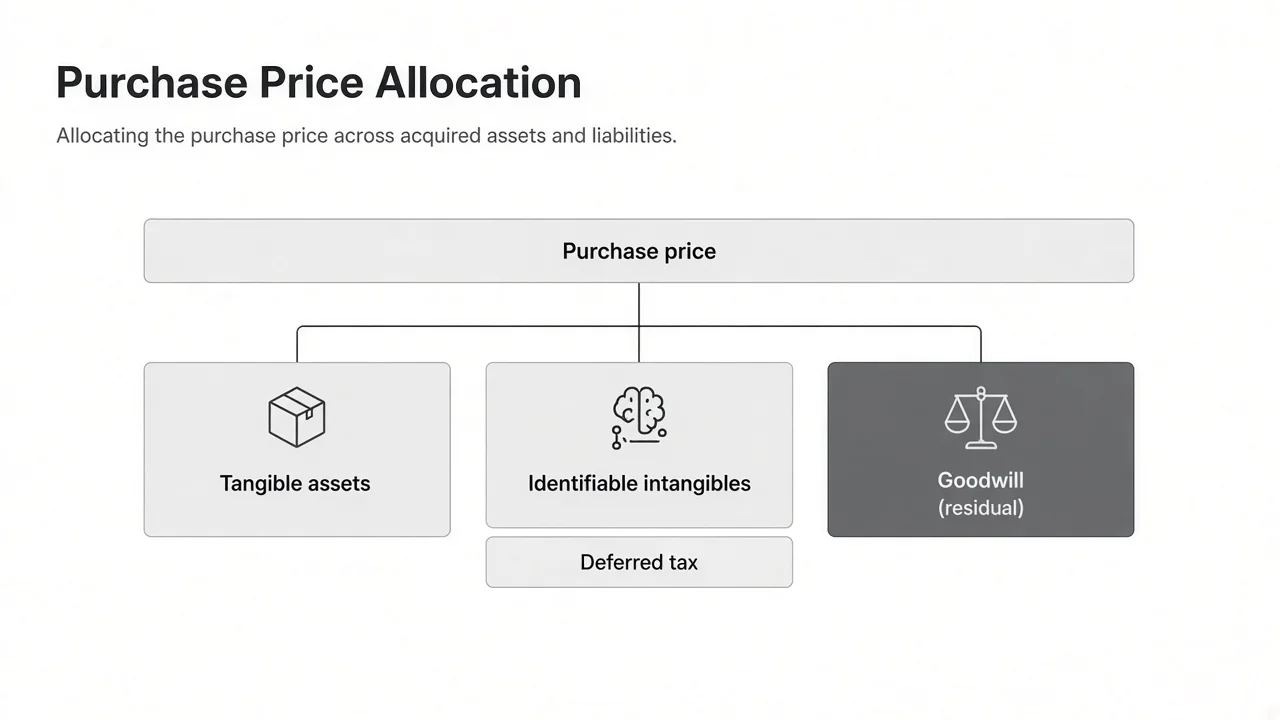
Purchase price allocation assigns a deal's price to every asset and liability at fair value and leaves goodwill as the remainder. The steps, the deferred tax math, and the tax-return version, with Kimberly-Clark's Kenvue filing.